Earliest deadline first and dynamic priorities

Fixed-priority scheduling gives each task one priority for its whole life. An obvious alternative is to let priority follow urgency: at every instant, run the job whose absolute deadline is closest. This rule, earliest deadline first (EDF), changes the relative priority of tasks from job to job, which is why it is called a dynamic-priority or, more precisely, a job-level fixed-priority scheduler. EDF has a remarkable property. On a single processor it is optimal: if any scheduling algorithm can meet all deadlines of a set of independent preemptive jobs, EDF can too. For periodic tasks with implicit deadlines this gives the simplest possible schedulability test, U ≤ 1, and lets a system use the whole processor. This lesson explains why EDF works, how to test it when deadlines are shorter than periods, how it behaves under overload, and why, despite its theoretical advantages, fixed priority still dominates industrial practice.

The question for the NS-5 is practical. The pedestrian-detection feature pushes the classifier to 11 ms and utilization to 0.812; lesson 4 showed that rate-monotonic scheduling still copes. A later radar upgrade might push utilization past 0.9. Maren asks Jonah whether switching the kernel to EDF, which the kernel supports as a configuration option, would buy enough headroom to be worth it.

The EDF rule and its optimality

Under EDF, every job carries its absolute deadline d = r + D. The scheduler keeps the ready jobs ordered by deadline and always runs the first one; when a new job is released with an earlier deadline than the running job, it preempts. Ties can be broken arbitrarily, for example by task index.

The optimality argument, due to Dertouzos in 1974, is an exchange argument. Take any schedule that meets all deadlines. Wherever it runs a job with a later deadline while a job with an earlier deadline is ready, swap the two pieces of execution. The earlier-deadline job now finishes no later than before, and the later-deadline job finishes no later than the earlier job's deadline did in the original schedule, which was before its own deadline. Repeating the swap transforms the schedule into the EDF schedule without ever causing a miss. Therefore, if any feasible schedule exists, the EDF schedule is feasible too.

For periodic tasks with implicit deadlines, Liu and Layland proved in 1973 that EDF meets every deadline if and only if:

The test is exact and needs nothing but utilization. With the 11 ms classifier the NS-5 has U = 0.812, comfortably schedulable under EDF; it would remain schedulable under EDF up to U = 1, while under rate-monotonic priorities a set with less harmonic periods could fail anywhere above 0.743.

RM and EDF side by side

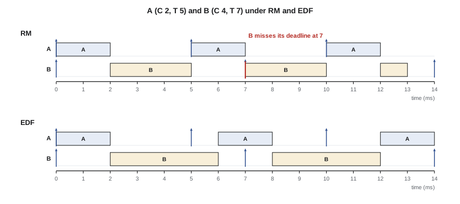
The textbook example that separates the two schedulers has two tasks: A with C = 2 and T = D = 5, and B with C = 4 and T = D = 7, in milliseconds. The utilization is 2/5 + 4/7 = 0.971, so EDF will meet every deadline. Under rate-monotonic priorities A always wins, and response-time analysis gives R_B = 4 + ceil(R_B/5) × 2, which iterates 4, 6, 8: the first job of B finishes at 8 ms, past its deadline at 7 ms. The simulator below runs both schedulers in 1 ms ticks over the 35 ms hyperperiod and prints a text Gantt chart, one character per millisecond. A late job is dropped at its deadline, as a firm-deadline system would do.

def simulate(tasks, policy, horizon):
    """tasks: (name, C, T, D) in integer ticks; returns timeline and misses"""
    jobs, line, misses = [], [], []
    for t in range(horizon):
        for i, (name, c, per, d) in enumerate(tasks):
            if t % per == 0:
                jobs.append([t + d, i, c, t])            # deadline, task, remaining, release
        for j in [j for j in jobs if j[0] <= t and j[2] > 0]:
            misses.append((tasks[j[1]][0], j[3], j[0]))
            jobs.remove(j)                                # drop the late job (firm deadline)
        ready = [j for j in jobs if j[2] > 0]
        if not ready:
            line.append(".")
            continue
        if policy == "RM":
            job = min(ready, key=lambda j: (tasks[j[1]][2], j[0]))
        else:
            job = min(ready, key=lambda j: (j[0], j[1]))
        job[2] -= 1
        line.append(tasks[job[1]][0][0])
        if job[2] == 0:
            jobs.remove(job)
    return "".join(line), misses

tasks = [("A", 2, 5, 5), ("B", 4, 7, 7)]
H = 35
print("U =", round(sum(c / t for _, c, t, _ in tasks), 3), " hyperperiod", H)
ruler = "".join(str(t // 10) if t % 10 == 0 else " " for t in range(H))
ticks = "".join(str(t % 10) for t in range(H))
for policy in ("RM", "EDF"):
    line, misses = simulate(tasks, policy, H)
    print(f"\n{policy}")
    print("      " + ruler)
    print("      " + ticks)
    print("      " + line)
    for name, rel, dl in misses:
        print(f"  {name} released at {rel} missed its deadline at {dl}")
    if not misses:
        print("  no deadline misses")

U = 0.971  hyperperiod 35

RM
      0         1         2         3    
      01234567890123456789012345678901234
      AABBBAABBBAAB.BAABBBAABBBAABBBAABB.
  B released at 0 missed its deadline at 7

EDF
      0         1         2         3    
      01234567890123456789012345678901234
      AABBBBAABBBBAABAABBBAABBBBAABBAABB.
  no deadline misses

The first rows of each chart are a ruler: tens on top, units below. Under RM, A runs at 0 to 2 ms, B at 2 to 5 ms, then A is released again at 5 ms and preempts B, which still needs 1 ms; when A finishes at 7 ms, B's deadline has passed and the job is dropped. Under EDF, at 5 ms the running job of B has deadline 7 while the new job of A has deadline 10, so B continues and finishes at 6 ms, and A runs at 6 to 8 ms, still well before its deadline. Over the whole hyperperiod EDF meets every deadline and leaves exactly 1 ms idle, which is the 3 % of capacity the utilization leaves free.

Constrained deadlines: the processor demand criterion

When some deadlines are shorter than periods, U ≤ 1 is still necessary but no longer sufficient, and the density test, Σ C_i/min(D_i, T_i) ≤ 1, is sufficient but often pessimistic. The exact test, due to Baruah, Rosier and Howell in 1990, is based on the demand bound function. For an interval of length L starting at a synchronous release, dbf(L) is the total execution time of all jobs that are both released and due within the interval:

A synchronous task set with U ≤ 1 is schedulable under EDF if and only if dbf(L) ≤ L for every L. The demand function only steps up at absolute deadlines, so it is enough to check the values of L that are deadlines, up to a bound such as the hyperperiod plus the largest deadline. Tighter bounds and faster algorithms exist; Zhang and Burns's quick processor-demand analysis, published in 2009, checks far fewer points by stepping backwards through the interval, and it is what practical tools use.

from math import gcd
from functools import reduce

tasks = [("SENSE", 1, 4, 3), ("FILTER", 2, 6, 4), ("ACT", 3, 10, 8)]   # C, T, D in ms

U = sum(c / t for _, c, t, _ in tasks)
dens = sum(c / min(t, d) for _, c, t, d in tasks)
H = reduce(lambda a, b: a * b // gcd(a, b), [t for _, _, t, _ in tasks])
print(f"U = {U:.3f}, density = {dens:.3f}, hyperperiod = {H}")

def dbf(L):
    return sum(max(0, (L - d) // t + 1) * c for _, c, t, d in tasks)

limit = H + max(d for _, _, _, d in tasks)
points = sorted({k * t + d for _, c, t, d in tasks for k in range(limit // t + 1) if k * t + d <= limit})
worst = min(points, key=lambda L: L - dbf(L))
bad = [L for L in points if dbf(L) > L]
for L in points[:8]:
    print(f"  L = {L:2d}  demand = {dbf(L):2d}  {'ok' if dbf(L) <= L else 'overload'}")
print(f"checked {len(points)} deadlines up to {limit}; tightest at L = {worst} with slack {worst - dbf(worst)}")
print("schedulable under EDF" if not bad else f"not schedulable: first overload at L = {bad[0]}")

U = 0.883, density = 1.208, hyperperiod = 60
  L =  3  demand =  1  ok
  L =  4  demand =  3  ok
  L =  7  demand =  4  ok
  L =  8  demand =  7  ok
  L = 10  demand =  9  ok
  L = 11  demand = 10  ok
  L = 15  demand = 11  ok
  L = 16  demand = 13  ok
checked 33 deadlines up to 68; tightest at L = 4 with slack 1
schedulable under EDF

The check examines 33 absolute deadlines up to 68 ms. The tightest point is L = 4 ms, with 1 ms of slack. The set is schedulable under EDF, even though its density of 1.208 would have rejected it. Under deadline-monotonic fixed priorities the same set fails. SENSE is first and FILTER meets its deadline with R = 2 + 1 = 3 ≤ 4, but for ACT the iteration R = 3 + ceil(R/4) + 2 ceil(R/6) runs 3, 6, 7, 9, and 9 ms exceeds its 8 ms deadline. Here EDF's ability to reorder jobs by deadline, rather than by task, is exactly what saves the set.

Overload and the domino effect

EDF's strength becomes a weakness when the system is overloaded. Under fixed priority, an overrun by a low-priority task can never delay a high-priority one; the damage is confined to tasks below the culprit. Under EDF, a job that overruns keeps its deadline, and as other jobs' deadlines approach they preempt it, or, once its deadline is the earliest, it runs ahead of everyone. In a transient overload EDF can therefore cause a cascade of misses across many tasks, called the domino effect, where a fixed-priority system would lose only its lowest-priority work. Firm-deadline systems can limit the damage by dropping jobs whose deadlines have passed, as the simulator above does, but the general cure is budget enforcement: the kernel limits each task to its declared execution time per period, as the constant bandwidth server of lesson 8 does.

Overload is not an exotic condition. Execution-time estimates can be wrong, interrupts can arrive in bursts, and hardware faults can cause retries. A design review should ask what happens when the analysis assumptions are violated, not just whether the analysis passes. For the NS-5, a burst of vehicles may make the classifier run longer than its bound, and under fixed priority the cost of that falls only on LOG and HOUSE, both of which have very large slack.

Other dynamic-priority schedulers

Least laxity first (LLF), also called least slack time first, runs the job with the smallest laxity, the time to its deadline minus its remaining execution time. LLF is also optimal on one processor and reacts earlier to jobs that are about to become late, but laxity changes continuously as jobs run, so two jobs with equal laxity can thrash, preempting each other at every tick. It is rarely used in practice. On multiprocessors, discussed in lesson 9, neither EDF nor LLF is optimal, and families such as Pfair and its successors take over the role of optimal schedulers.

Why fixed priority still dominates

If EDF is optimal and uses the whole processor, why do most real-time kernels and almost all certified systems use fixed priority? Buttazzo compared the two carefully in 2005 and found that several common objections to EDF are weaker than they seem. EDF typically causes fewer preemptions than RM, because a job close to finishing with a near deadline is not preempted by a fresh job with a distant one, and its run-time overhead with a good priority queue is modest. But real advantages of fixed priority remain. Interrupt controllers implement fixed priorities in hardware, so interrupt handlers are fixed-priority whatever the kernel does. Behaviour under overload is predictable and confined. Priorities are easy to explain, review and certify, and decades of tools, standards and engineering experience assume them. Many protocols for shared resources and networks, such as the CAN arbitration of lesson 11, are inherently fixed-priority.

For the NS-5, Jonah's recommendation is to stay with fixed priority. Response-time analysis shows the planned features fit with all deadlines met, the critical scaling factor of about 1.6 leaves margin for growth, and the overload behaviour of fixed priority suits a product where radar frames must never be sacrificed for logging. EDF remains a valid choice for systems with high utilization and well-enforced budgets, such as multimedia processing and soft real-time servers, and an increasing number of general-purpose kernels offer it as a scheduling class for exactly that purpose.