
CMP-440 · Lesson 2 of 12 · 22 min
Task models for real-time systems
Before anyone can prove that a system meets its deadlines, the system has to be described in a form that analysis can work on. Real-time scheduling theory does this with task models: small sets of numbers that capture how often each activity runs, how long it can take and when it must finish. A task model deliberately throws information away. It does not care what the classifier computes, only that it needs at most 6 ms of processor time every 25 ms and must finish within 25 ms of its release. That abstraction is what makes the theory of the next lessons possible, and choosing the right abstraction is a design skill in its own right. This lesson defines the standard periodic and sporadic task models, the parameters that describe them, the derived quantities such as utilization and hyperperiod, and the assumptions on which every later result rests.
Jonah's first deliverable on the NS-5 is a task table: a single page listing every activity in the firmware with its timing parameters, signed off by Maren Holt and hardware lead Ines Carvalho. Every schedulability argument in this course starts from that table, and every change to the firmware that alters a number in it must trigger a new analysis.
Tasks and jobs
A task is a recurring activity, such as 'process a radar frame' or 'send CAN status'. Each occurrence of a task is a job. A task is written τ_i, with i an index, and its k-th job is often written J_(i,k). Each job has a release time r, the instant it becomes ready to run; an execution time, the processor time it needs; a finishing time f; and an absolute deadline d. Its response time is f − r, the time from release to completion, and it meets its deadline if f ≤ d.
A job may be preempted, meaning suspended in the middle of its execution so that a more urgent job can run, and resumed later. Most of the theory in this course assumes fully preemptive scheduling, in which a job can be preempted at any instant at negligible cost. Lesson 6 looks at what preemption really costs on a processor, and lesson 7 at what happens when a job holds a shared resource while preempted.
The periodic task model
In the periodic task model introduced by Liu and Layland in 1973, each task τ_i is described by a small tuple of parameters. These are the variables used throughout the rest of the course.
| Symbol | Name | Meaning |
|---|---|---|
| C_i | Worst-case execution time (WCET) | The largest processor time any job of the task can need when running alone |
| T_i | Period | The fixed interval between successive releases |
| D_i | Relative deadline | The time after each release by which the job must finish |
| Φ_i | Phase or offset | The release time of the first job |
| J_i | Release jitter | The largest delay between the nominal arrival and the actual release |
| U_i = C_i / T_i | Utilization | The fraction of the processor the task needs in the long run |
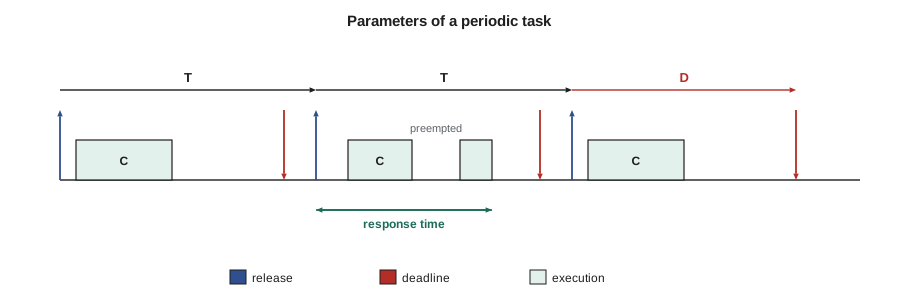
Deadlines are classified by their relation to periods. A task has an implicit deadline if D_i = T_i, so each job must finish before the next is released; this is the case Liu and Layland analyzed and the case of the NS-5's radar frame. A constrained deadline has D_i ≤ T_i, typical of control loops where the actuator must be updated early in each period to limit delay. An arbitrary deadline may exceed the period, so that several jobs of the same task can be pending at once; this occurs in pipelines and in network message streams. The analysis becomes harder at each step, and lesson 4 shows how response-time analysis handles all three.
Phase matters too. If all tasks have phase zero, they are synchronous, and they are all released together at time zero. Liu and Layland showed that for fixed-priority scheduling this simultaneous release, the critical instant, produces the worst-case response time of every task when tasks are independent. Analysis therefore usually assumes it, even if the real system staggers its tasks, because it is safe: any other phasing can only be better.
Sporadic and aperiodic activities
Not every activity is triggered by a clock. A sporadic task is released by events, such as an interrupt or an incoming message, but with a known minimum interarrival time between releases. In the analysis, T_i is that minimum separation, and the worst case is the one where events arrive as fast as allowed. A sporadic task with minimum separation T_i therefore imposes no more load than a periodic task with period T_i, which is why most results for periodic tasks carry over unchanged. An aperiodic activity has no such bound: a button press, a configuration command from the service port, an operator query. Aperiodic work cannot be guaranteed on its own; it must be confined to a budget that protects the periodic work, which is the subject of lesson 8.
Minimum interarrival times do not appear by themselves. If a sensor interrupt can fire on every edge of a noisy signal, its minimum separation is effectively zero and no analysis can bound it. Real-time designs enforce separation in hardware or in the driver, for example by disabling an interrupt for a fixed time after it fires, or by rate-limiting events into a queue. The NS-5's CAN receive interrupt is bounded by the bus itself: at 500 kbit/s a frame cannot arrive more often than once every 94 bit times or so, even with the shortest possible frame.
Derived quantities
Three quantities derived from the task parameters appear in every analysis. The total utilization U is the sum of the task utilizations. It is the long-run fraction of processor time the task set demands, and no scheduler on one processor can meet every deadline if U > 1, because there is simply not enough processor time.
The density replaces T_i with min(D_i, T_i) in each term. It matters for constrained deadlines, where a task must finish its work in a window shorter than its period: a task with C = 2 ms, T = 10 ms and D = 4 ms has utilization 0.2 but density 0.5. A density at most 1 is sufficient, but not necessary, for schedulability under earliest deadline first.
The hyperperiod H is the least common multiple of the periods. With synchronous release and deadlines no longer than periods, the pattern of releases repeats every H, so a schedule that meets every deadline over one hyperperiod meets every deadline forever. The hyperperiod is the planning horizon of a cyclic executive in lesson 3 and the simulation length used by the simulators later in the course. It can be huge: periods of 7, 11, 13 and 17 ms give a hyperperiod of 17,017 ms, which is why designers often choose harmonic periods, each a multiple of the next shorter one.
The NS-5 task table
Jonah's table for the NS-5 lists five periodic tasks. The radar task, RADAR, processes each frame within the frame period. The CAN service task, CANTX, sends status and diagnostic messages and services the transmit queue. The classifier, CLASS, runs every four frames. The logger, LOG, writes counts and events to the ferroelectric memory, and the housekeeping task, HOUSE, reads the battery and temperature sensors and updates the service display. Interrupt handlers, which are short and bounded, are treated separately in lesson 6.
| Task | C (ms) | T (ms) | D (ms) | U |
|---|---|---|---|---|
| RADAR | 1.2 | 6.25 | 6.25 | 0.192 |
| CANTX | 0.8 | 10 | 10 | 0.080 |
| CLASS | 6.0 | 25 | 25 | 0.240 |
| LOG | 8 | 100 | 100 | 0.080 |
| HOUSE | 20 | 1000 | 1000 | 0.020 |
| Total | 0.612 |
The total utilization of 0.612 says that, in the long run, the processor is busy 61.2 % of the time with periodic work. It does not yet say that every deadline will be met; lesson 4 answers that question. The code below computes the derived quantities and lists the releases in the first 25 ms.
from math import gcd
from functools import reduce

# name, C, T, D in microseconds so that the arithmetic stays exact
tasks = [("RADAR", 1_200, 6_250, 6_250), ("CANTX", 800, 10_000, 10_000),
         ("CLASS", 6_000, 25_000, 25_000), ("LOG", 8_000, 100_000, 100_000),
         ("HOUSE", 20_000, 1_000_000, 1_000_000)]

U = sum(c / t for _, c, t, _ in tasks)
density = sum(c / min(d, t) for _, c, t, d in tasks)
H = reduce(lambda a, b: a * b // gcd(a, b), [t for _, _, t, _ in tasks])
jobs = sum(H // t for _, _, t, _ in tasks)

print(f"total utilization U = {U:.3f}, density = {density:.3f}")
print(f"hyperperiod H = {H/1000:.0f} ms, jobs per hyperperiod = {jobs}")
for name, c, t, d in tasks:
    print(f"  {name:6s} U = {c/t:.3f}  jobs per H = {H//t}")

print("releases in the first 25 ms:")
events = sorted((k * t, name) for name, c, t, d in tasks for k in range(25_000 // t + 1) if k * t <= 25_000)
for when, name in events:
print(f" {when/1000:6.2f} ms {name}")total utilization U = 0.612, density = 0.612
hyperperiod H = 1000 ms, jobs per hyperperiod = 311
RADAR U = 0.192 jobs per H = 160
CANTX U = 0.080 jobs per H = 100
CLASS U = 0.240 jobs per H = 40
LOG U = 0.080 jobs per H = 10
HOUSE U = 0.020 jobs per H = 1
releases in the first 25 ms:
0.00 ms CANTX
0.00 ms CLASS
0.00 ms HOUSE
0.00 ms LOG
0.00 ms RADAR
6.25 ms RADAR
10.00 ms CANTX
12.50 ms RADAR
18.75 ms RADAR
20.00 ms CANTX
25.00 ms CLASS
25.00 ms RADARThe hyperperiod is exactly 1 s, because every period divides 1,000 ms, and it contains 311 jobs. At time zero all five tasks are released together, the critical instant. RADAR is released again at 6.25, 12.5, 18.75 and 25 ms, CANTX at 10 and 20 ms, and CLASS again at 25 ms. Harmonic or nearly harmonic periods like these keep the hyperperiod short and, as lesson 4 shows, also raise the utilization a fixed-priority scheduler can guarantee.
Precedence, chains and end-to-end timing
Tasks in real systems are rarely independent. The classifier needs the results of four radar frames; the CAN message carries the classifier's decision; the logger records what the classifier decided. Such dependencies form chains. Two ways of connecting the tasks of a chain lead to very different timing. In a synchronized, or event-triggered, chain each task releases the next when it finishes, so the end-to-end latency is the sum of the response times. In an asynchronous, or sampling, chain each task runs on its own period and reads the latest data its predecessor left in a shared buffer. Each link can then add up to one period of the reader plus its response time, which is exactly the calculation of lesson 1's worked example.
Asynchronous chains are common because they decouple tasks and are easy to analyze one task at a time, but their end-to-end latency can be surprisingly large. The automotive industry calls the two quantities data age, the delay from a sensor reading to the output that uses it, and reaction time, the delay from an external event to the first output that reflects it. Both must be computed as part of the end-to-end requirement, and both depend on the periods and response times of every task in the chain.
Worked problem
Reaction time of the radar-to-classifier chain
RADAR runs every 6.25 ms with a worst-case response time of 1.2 ms. CLASS runs every 25 ms and reads the most recent four frame results when it starts. If CLASS has a worst-case response time of 9.2 ms, what is the worst-case reaction time from a vehicle first appearing in a radar frame to CLASS producing a decision that includes that frame?
Show solution
- In the worst case the vehicle appears just after a RADAR release, so it is captured in the next frame: a wait of up to one radar period, 6.25 ms, plus the frame's processing response time of 1.2 ms.
- \[ t_{\text{frame ready}} = 6.25 + 1.2 = 7.45\ \text{ms}\]
- The frame result is then waiting for CLASS, which in the worst case has just started and missed it, so it waits one CLASS period and the next job's full response time.
- \[ t_{\text{reaction}} = 7.45 + 25 + 9.2 = 41.65\ \text{ms}\]
Answer: The worst-case reaction time is 41.65 ms. A synchronized chain, where RADAR releases CLASS directly after the fourth frame, would remove most of the 25 ms sampling wait.
Assumptions behind the model
Every guarantee in the following lessons holds only under the assumptions of the model, so it is worth stating them plainly. The classical periodic model of Liu and Layland assumes a single processor; independent tasks that do not share resources or wait for each other; implicit deadlines; zero release jitter; known worst-case execution times; negligible overhead for scheduling and context switches; and tasks that never suspend themselves voluntarily, for example to wait for I/O. Real systems violate almost all of these.
The response of the theory has been to relax the assumptions one at a time and extend the analysis, rather than to abandon the model. Lesson 4 adds constrained deadlines and release jitter. Lesson 6 adds kernel overheads. Lesson 7 adds shared resources and blocking. Lesson 8 adds aperiodic work. Lesson 9 adds multiple processors, and lesson 10 asks where the C_i values come from in the first place. The practical lesson for a designer is that the task table is not just a list of numbers. It is a contract. If a developer adds a blocking file write to the housekeeping task, or a new interrupt source, or a cache-unfriendly data structure to the classifier, the contract changes and the analysis must be repeated.
Self-suspension deserves special mention because it is easy to introduce by accident. A task that starts a DMA transfer and then waits on a semaphore for completion is suspended during the transfer, and its job no longer behaves like one contiguous block of execution. Treating the suspension time as if it were execution time is safe but pessimistic. Ignoring it is unsafe, because a suspended higher-priority task can later resume and impose more interference on lower-priority tasks than the classical analysis expects. Several published analyses of self-suspending tasks were later found to be flawed for exactly this reason, which is a good argument for keeping suspensions out of hard real-time tasks where possible.
Common mistakes
MistakeUsing the average execution time for C.
InsteadC is the worst-case execution time; analysis with averages proves nothing about the worst case.
MistakeTreating an interrupt-driven task with no minimum separation as sporadic.
InsteadA sporadic task needs an enforced minimum interarrival time; otherwise it is aperiodic.
MistakeAssuming staggered phases make analysis optimistic.
InsteadAnalysis assumes the critical instant, which is safe; staggering only helps if it is guaranteed.
MistakeForgetting the sampling waits in asynchronous chains.
InsteadEach link can add up to a reader period plus its response time to the end-to-end latency.
MistakeLeaving the task table unchanged after a code change.
InsteadThe table is a contract; any change to execution time, period or blocking requires a new analysis.
Summary and key terms
- A task is a recurring activity; each occurrence is a job with a release, execution time, finish and deadline.
- The periodic model describes each task by C, T, D and optionally phase and jitter.
- Deadlines are implicit (D = T), constrained (D ≤ T) or arbitrary.
- Sporadic tasks have a minimum interarrival time and can be analyzed like periodic ones; aperiodic tasks cannot.
- Utilization, density and hyperperiod summarize a task set; U > 1 is never schedulable on one processor.
- Chains of tasks have end-to-end latencies that include sampling waits in asynchronous designs.
- The model rests on explicit assumptions that later lessons relax one at a time.
- Task
- A recurring activity in a real-time system, described by timing parameters.
- Job
- One occurrence of a task.
- Worst-case execution time (WCET)
- The largest processor time a job of a task can need when running alone.
- Implicit deadline
- A relative deadline equal to the period.
- Sporadic task
- An event-released task with a known minimum interarrival time.
- Utilization
- The long-run fraction of processor time a task or task set needs.
- Hyperperiod
- The least common multiple of the task periods, after which the release pattern repeats.
- Critical instant
- A release pattern that produces the worst-case response time of a task.
Practice problems
Work each problem on paper first, then reveal the answer to check.
A task has C = 3 ms, T = 20 ms and D = 12 ms. Give its utilization and its density term.
Show answer
U = 3/20 = 0.15; density term 3/12 = 0.25.
What is the hyperperiod of periods 4, 6 and 10 ms?
Show answer
lcm(4, 6, 10) = 60 ms.
If CLASS were released directly by RADAR after every fourth frame, what would the reaction time in the worked example become, ignoring any extra queuing?
Show answer
About 7.45 + up to three more frames (18.75 ms) + 9.2 ms, or 35.4 ms; the sampling wait of 25 ms becomes a wait for the remaining frames.
Why is a sporadic task with minimum separation 10 ms no worse for analysis than a periodic task with period 10 ms?
Show answer
Its worst case is releases exactly 10 ms apart, which is the periodic pattern; any slower arrivals add less load.
Lesson quiz · 5 questions
Score 60% or more to complete this lesson.
Create a free account to save your progress, take quizzes and earn a certificate.