Timing analysis and worst-case execution time

Every schedulability test in this course takes the worst-case execution times C_i as given. They are not given. Someone has to find them, and the result has to be an upper bound: an underestimate makes every guarantee built on it worthless, while a large overestimate wastes the processor and may make a feasible design look infeasible. Finding the worst-case execution time (WCET) of a piece of code is hard in general, since it requires knowing the longest path through the program, the input data that drives it there and the behaviour of the processor's pipelines, caches and buses along the way. This lesson explains why execution times vary, how they are measured, how static analysis bounds them, why combining the two is common practice and how design choices make the problem easier.

Lesson 8 used two execution-time estimates for the NS-5 classifier: a measured value of 6 ms and a conservative bound of 9 ms required by the safety assessor. This lesson shows where both numbers came from, and why the assessor would not accept the measured value alone.

Why execution times vary

The execution time of one job depends on the path taken through the code, which depends on input data: how many radar targets are in the frame, whether any is large enough to need extra features, whether a pedestrian-like return triggers the slower neural-network classifier. It depends on the state of the processor when the job starts: what is in the instruction and data caches, the branch predictor's history, the contents of write buffers. And on a multicore processor or a system with DMA, it depends on what else is using the memory system at the same time, as lesson 9 discussed. Most jobs take close to a typical value; a few take much longer. The resulting distribution has a long tail on the right, and the WCET is the far end of that tail.

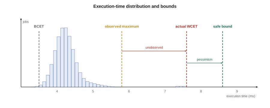
Three quantities matter. The best-case execution time (BCET) is the shortest any job can take; it matters for jitter and for some network analyses. The actual WCET is the longest any job can take, which is usually unknown. A WCET bound is a value proven or argued to be at least the actual WCET. Analysis aims for bounds that are both safe, never below the actual WCET, and tight, not far above it.

Measurement-based timing analysis

The most common approach in industry is measurement: run the code on the target hardware many times with as many different inputs as possible, record the longest execution time observed, the high-water mark, and add an engineering margin, often 20 to 50 %. Measurements are made with hardware cycle counters, with trace hardware that records branch history, or by toggling a GPIO pin at the start and end of the code and capturing it with a logic analyzer. On RISC-V, the mcycle counter counts processor cycles and minstret counts instructions retired; both are 64-bit control and status registers readable from machine mode.

#include <stdint.h>

static inline uint64_t read_mcycle(void)
{
#if __riscv_xlen == 32
    uint32_t hi, lo, hi2;
    do {                                   /* read hi, lo, hi again in case lo wrapped */
        __asm__ volatile ("csrr %0, mcycleh" : "=r"(hi));
        __asm__ volatile ("csrr %0, mcycle"  : "=r"(lo));
        __asm__ volatile ("csrr %0, mcycleh" : "=r"(hi2));
    } while (hi != hi2);
    return ((uint64_t)hi << 32) | lo;
#else
    uint64_t c;
    __asm__ volatile ("csrr %0, mcycle" : "=r"(c));
    return c;
#endif
}

static uint64_t class_hwm;                  /* high-water mark in cycles */

void classify_frame_set(void)
{
    uint64_t t0 = read_mcycle();
    run_classifier();
    uint64_t dt = read_mcycle() - t0;
    if (dt > class_hwm) class_hwm = dt;     /* reported over the service port */
}

Measurement has real strengths. It captures the actual hardware, including effects no model describes, and it is cheap to run continuously, during development, in system tests and even in deployed products, as the NS-5 does by reporting its high-water marks over the service port. Its weakness is coverage. The longest path may need a rare combination of inputs that testing never produces, and the worst hardware state may need a particular cache and pipeline history. The simulation below models the classifier's execution time with a routine part, an occasional extra cost for trucks and a very rare slow path, which a static analysis of the code bounds at 8.6 ms, and shows what a measurement campaign of increasing length would conclude.

import random
random.seed(10)

# Execution time of one classifier job in microseconds. Most frames are routine;
# rarely, several large vehicles and a pedestrian appear together and the slow path runs.
def classifier_time():
    t = random.gauss(4_200, 250)                 # routine frames
    if random.random() < 0.02:
        t += random.uniform(500, 900)            # a truck: extra features
    if random.random() < 1e-5:
        t += 3_200                               # rare combination: neural network path for many targets
    return t

TRUE_WCET_BOUND = 8_600                          # from static analysis of the code, microseconds
for runs in (1_000, 10_000, 100_000, 1_000_000):
    hwm = max(classifier_time() for _ in range(runs))
    print(f"{runs:9,d} runs: high-water mark {hwm/1000:5.2f} ms   "
          f"+20 % margin {1.2*hwm/1000:5.2f} ms   static bound {TRUE_WCET_BOUND/1000:4.2f} ms")

    1,000 runs: high-water mark  5.44 ms   +20 % margin  6.53 ms   static bound 8.60 ms
   10,000 runs: high-water mark  5.83 ms   +20 % margin  7.00 ms   static bound 8.60 ms
  100,000 runs: high-water mark  7.56 ms   +20 % margin  9.07 ms   static bound 8.60 ms
1,000,000 runs: high-water mark  8.10 ms   +20 % margin  9.72 ms   static bound 8.60 ms

After 1,000 or 10,000 runs, the high-water mark is 5.44 or 5.83 ms, and even with a 20 % margin the estimate of 6.53 or 7.00 ms is below the rare slow path. Only after 100,000 runs does the slow path appear, raising the high-water mark to 7.56 ms. A product that classifies 40 vehicle windows per second performs 100,000 runs in well under an hour, so the slow path will occur in service, probably many times a day across a city. The measured 6 ms used for C(LO) is a good description of normal operation; it is not a bound. This is why measurement alone is accepted only for lower-criticality functions, and why safety standards expect either static analysis or a strong argument that the measurements covered the worst paths and hardware states.

Measurement-based probabilistic timing analysis tries to extrapolate from measurements using extreme value theory, fitting a distribution to the largest observed values and estimating the execution time that will be exceeded with a probability below, say, 10^(−9) per job. The method is attractive, but its validity rests on assumptions that are hard to check on real processors: that runs are independent and identically distributed, and that the measured runs represent all the paths and hardware states that can occur. A rare path that never appeared in the measurements, like the one in the simulation, is invisible to any extrapolation.

Static timing analysis

Static analysis bounds the WCET without running the code. It works on the compiled binary, because execution time depends on the actual instructions and their addresses, and follows a standard sequence of steps. First, control-flow reconstruction builds the control-flow graph of basic blocks from the binary. Second, flow analysis finds loop bounds and infeasible paths, partly automatically and partly from annotations, called flow facts, that the developer supplies: 'this loop runs at most 64 times', 'the network branch runs for at most 8 targets per frame'. Third, processor behaviour analysis computes a bound on the execution time of each basic block, using abstract interpretation to classify each memory access as an always-hit, always-miss or unknown for each cache level and modelling the pipeline. Fourth, path analysis combines the block bounds into a bound on the whole program.

The usual method for the last step is the implicit path enumeration technique (IPET), introduced by Li and Malik in 1995. Each basic block i gets an execution count x_i and a cost c_i, flow conservation constraints say that the count of each block equals the sum of the counts on its incoming edges, loop bounds and flow facts become further linear constraints, and an integer linear program maximizes the total cost:

The classifier's target-scoring loop gives a small illustration. Each of up to 64 iterations runs a 6-cycle loop overhead and a 12-cycle gate check, then either skips the target at 5 cycles or computes features at 220 cycles, followed by either a decision tree at 150 cycles or the neural network at 900 cycles. With the loop bound alone, the worst path runs the network for all 64 targets. The flow fact that the network runs for at most 8 targets per frame, which the code enforces with a counter, cuts the bound sharply. The code below finds the IPET maximum by enumerating the feasible counts, which is practical for so small a problem; real tools use an ILP solver.

# Implicit path enumeration (IPET) for the classifier's inner loop, solved by enumeration.
# Block costs in cycles from pipeline analysis; the loop runs at most 64 times per job.
COST = {"entry": 40, "loop": 6, "gate": 12, "skip": 5, "features": 220,
        "tree": 150, "network": 900, "exit": 30}
MAX_TARGETS = 64
MAX_NETWORK = 8          # flow fact: the network path runs for at most 8 targets per frame
CLOCK_MHZ = 48

def wcet(max_network):
    best = None
    for nn in range(0, min(max_network, MAX_TARGETS) + 1):
        for feat in range(nn, MAX_TARGETS + 1):         # every network or tree call follows features
            tree = feat - nn
            skip = MAX_TARGETS - feat
            cycles = (COST["entry"] + COST["exit"]
                      + MAX_TARGETS * (COST["loop"] + COST["gate"])
                      + skip * COST["skip"] + feat * COST["features"]
                      + tree * COST["tree"] + nn * COST["network"])
            if best is None or cycles > best[0]:
                best = (cycles, nn, tree, skip)
    return best

for label, limit in (("loop bound only", MAX_TARGETS), ("with flow fact", MAX_NETWORK)):
    cycles, nn, tree, skip = wcet(limit)
    print(f"{label:16s}: {cycles:6d} cycles = {cycles/CLOCK_MHZ/1000:5.2f} ms "
          f"(network {nn}, tree {tree}, skipped {skip})")

loop bound only :  72902 cycles =  1.52 ms (network 64, tree 0, skipped 0)
with flow fact  :  30902 cycles =  0.64 ms (network 8, tree 56, skipped 0)

With only the loop bound, the WCET bound is 72,902 cycles, or 1.52 ms at 48 MHz. With the flow fact, it is 30,902 cycles, 0.64 ms, with the network on 8 targets and the decision tree on the other 56. The flow fact is not an assumption about traffic: it is a property of the code, enforced by a counter, and the analysis is safe only because the code really enforces it. Applied to the whole classifier, the same process gives the bound of 8.6 ms used above, and the assessor's C(HI) of 9 ms adds a small margin for the remaining uncertainty in the hardware model.

Hardware that is hard to analyze

Static analysis is only as good as its model of the processor. Simple in-order pipelines with scratchpad or tightly coupled memories, like the NS-5's microcontroller, can be modelled precisely, and the bounds are typically within 10 to 30 % of the actual WCET. Out-of-order pipelines, complex cache replacement policies, speculative execution and shared multicore resources are much harder. Some processors also show timing anomalies, in which a locally faster event, such as a cache hit instead of a miss, leads to a globally slower execution, because it changes the order in which instructions compete for resources later. Timing anomalies mean an analysis cannot simply assume the locally worst case at each step; it must explore the alternatives. Processors free of such anomalies are said to be timing-compositional, and they make analysis far simpler.

Preemption also affects execution time. A preempted task may find its cache contents evicted when it resumes, and the extra misses, called cache-related preemption delay (CRPD), must be added to the response-time analysis, usually as an extra cost per preemption. Analyses compute which cache blocks are useful to the preempted task and which the preempting task can evict, and bound the delay by the overlap. On the NS-5, tightly coupled memory removes most of this cost, which is one reason Jonah's overhead model of lesson 6 could ignore it.

Designing for analyzability

The most effective way to get good WCET bounds is to write code that has them. Loops should have bounds that are visible, either as constants or as annotations backed by checks. Recursion should be avoided or bounded. Data-dependent paths should be few and balanced where possible; a single-path programming style, in which both sides of a branch are computed and the result selected, gives a constant execution time at the cost of always doing the slower work. Dynamic memory allocation, virtual dispatch through function pointers chosen at run time and calls into libraries without timing information all hinder analysis. Hardware choices matter just as much: scratchpads instead of caches for critical code, cache locking, simple pipelines and predictable buses. Research processors designed for timing predictability go further, with time-division memory arbitration and deterministic pipelines.

In practice, industrial projects combine methods. Static analysis bounds the most critical code. Measurements, with path coverage analysis, check that the bounds are plausible and catch errors in annotations; a measurement that exceeds a static bound reveals a mistake in the model. Continuous high-water-mark monitoring in deployed systems detects when reality departs from the analysis, which on the NS-5 triggers the mixed-criticality mode switch of lesson 8 and a log entry that the firmware team reviews.