Linear regression and regularization

Linear regression is the oldest and still one of the most useful learning methods. Legendre and Gauss developed least squares around 1805 to fit the orbits of comets and asteroids, and today linear models price insurance, forecast demand, calibrate sensors and serve as the baseline that every fancier model must beat. They also expose, in a setting simple enough to solve exactly, every theme of this course: a loss function, an optimization problem, a probabilistic interpretation, overfitting, and its cure by regularization.

STAT-151 treated regression as a tool for inference: confidence intervals for coefficients, hypothesis tests, checking residual plots. This lesson takes the machine learning view, in which the coefficients are a means to an end and the question is how well the fitted model predicts new cases. The two views share the same mathematics and differ mainly in what they report. AI-210 develops the underlying linear algebra, including projections and the singular value decomposition, in more depth.

The model and the least squares objective

A linear regression model predicts a real-valued output as a weighted sum of the input features plus an intercept:

where in the second form we have appended a constant feature \(x_0 = 1\) so that the intercept \(w_0\) is just another weight. Stack the n training inputs as rows of an \(n \times (p+1)\) design matrix X and the targets as a vector y. Empirical risk minimization with squared loss chooses the weights that minimize the residual sum of squares:

The model is linear in the weights, not necessarily in the original inputs. Nothing stops us from including \(x^2\), \(\log x\), interaction terms \(x_1 x_2\) or indicator variables for categories as features. The polynomial fits of lesson 2 were linear regressions on the features \(1, x, x^2, \ldots\). Feature construction, discussed in lesson 10, is how linear models capture curved relationships.

The normal equations

J is a convex quadratic in w, so its minimum is where the gradient vanishes. Differentiating,

These are the normal equations. If \(X^{\top} X\) is invertible, which requires at least as many examples as weights and no exact linear dependence among the features, the solution is unique: \(\hat{\mathbf{w}} = (X^{\top} X)^{-1} X^{\top} \mathbf{y}\). The name comes from geometry: the fitted vector \(X \hat{\mathbf{w}}\) is the orthogonal projection of y onto the column space of X, so the residual vector is normal (perpendicular) to every column. In code, one should never form the inverse explicitly; solving the linear system, or better still using a QR or singular value decomposition as numpy.linalg.lstsq does, is faster and numerically more stable.

Solving the normal equations costs about \(np^2 + p^3\) operations. That is trivial for a few dozen features and becomes expensive for hundreds of thousands, which is one reason iterative methods matter.

Gradient descent

Gradient descent starts from some weights and repeatedly steps downhill: \(\mathbf{w} \gets \mathbf{w} - \eta \nabla J(\mathbf{w})\), where the learning rate \(\eta\) controls the step size. For least squares the objective is convex, so with a small enough step size gradient descent converges to the global minimum. How fast it converges depends on the conditioning of \(X^{\top} X\): if one feature is measured in square metres (values in the hundreds) and another in years, the loss surface is a long narrow valley, and gradient descent zigzags. Standardizing each feature to mean 0 and standard deviation 1 makes the valley rounder and lets a single learning rate work for all weights.

Stochastic gradient descent (SGD) estimates the gradient from a single example or a small mini-batch rather than the full data set, which makes each step far cheaper and lets the method scale to data that do not fit in memory. SGD and its variants train essentially every neural network; AI-310 analyses their convergence. For linear regression on modest data the closed form is usually preferable, but the program below shows that the two approaches agree.

# Invented data: sale prices of 200 homes in a mid-sized Canadian city.
import numpy as np
rng = np.random.default_rng(367)
n = 200
area = rng.uniform(70, 260, n)                  # floor area, square metres
age = rng.uniform(0, 60, n)                     # years since built
dist = rng.uniform(1, 25, n)                    # km to downtown
price = 120 + 2.4 * area - 1.1 * age - 6.0 * dist + rng.normal(0, 40, n)   # thousands of dollars
X = np.column_stack([np.ones(n), area, age, dist])   # first column of ones gives the intercept
names = ["intercept", "area (per m2)", "age (per year)", "distance (per km)"]

# 1. closed form: solve the normal equations (X^T X) w = X^T y
w_closed = np.linalg.solve(X.T @ X, X.T @ price)

# 2. gradient descent on the mean squared error, after standardizing the features
mu, sd = X[:, 1:].mean(axis=0), X[:, 1:].std(axis=0)
Z = np.column_stack([np.ones(n), (X[:, 1:] - mu) / sd])
w = np.zeros(4); lr = 0.1
for step in range(500):
    grad = 2 / n * Z.T @ (Z @ w - price)
    w -= lr * grad
w_gd = np.concatenate([[w[0] - np.sum(w[1:] * mu / sd)], w[1:] / sd])   # undo the scaling

for name, a, b in zip(names, w_closed, w_gd):
    print(f"{name:18} closed form {a:9.3f}   gradient descent {b:9.3f}")
resid = price - X @ w_closed
print(f"training RMSE {np.sqrt(np.mean(resid ** 2)):.1f} thousand; R^2 = {1 - resid.var() / price.var():.3f}")

intercept          closed form   133.513   gradient descent   133.513
area (per m2)      closed form     2.319   gradient descent     2.319
age (per year)     closed form    -1.110   gradient descent    -1.110
distance (per km)  closed form    -5.748   gradient descent    -5.748
training RMSE 39.6 thousand; R^2 = 0.923

Both methods recover essentially the same weights, close to the values used to generate the data: each extra square metre adds about 2.3 thousand dollars, each year of age subtracts about 1.1 thousand, and each kilometre from downtown about 6 thousand. The training RMSE of about 40 thousand dollars matches the noise we built in; with real data you would not know the noise level and would estimate it from held-out residuals.

The probabilistic view

Least squares has a second justification. Suppose the targets are generated as \(y_i = \mathbf{w}^{\top} \mathbf{x}_i + \varepsilon_i\) with independent Gaussian noise \(\varepsilon_i \sim \mathcal{N}(0, \sigma^2)\). The likelihood of the weights is the probability of the observed targets:

Taking the negative logarithm turns the product into a sum, and every term not involving w is a constant. Maximizing the likelihood is therefore the same as minimizing the sum of squared residuals. This maximum likelihood estimate (MLE) view explains when least squares is the right choice, namely when errors are roughly Gaussian and of constant variance, and what to do otherwise. Heavy-tailed noise suggests absolute or Huber loss. Counts suggest Poisson regression. Binary outcomes suggest the logistic model of lesson 4. All of these are generalized linear models, which AI-320 treats in a Bayesian framework.

When least squares overfits

With many features relative to examples, least squares has high variance. When features are strongly correlated, \(X^{\top} X\) is nearly singular; tiny changes in the data swing the weights wildly, with large positive and negative weights on correlated features cancelling each other on the training data and failing elsewhere. When there are more features than examples, \(X^{\top} X\) is singular and infinitely many weight vectors fit the training data perfectly. Gene expression data with 20,000 genes and 200 patients, text with a feature per word, and the polynomial of degree 15 in lesson 2 are all examples.

Ridge regression

Ridge regression, introduced by Arthur Hoerl and Robert Kennard in 1970, adds a penalty on the squared size of the weights:

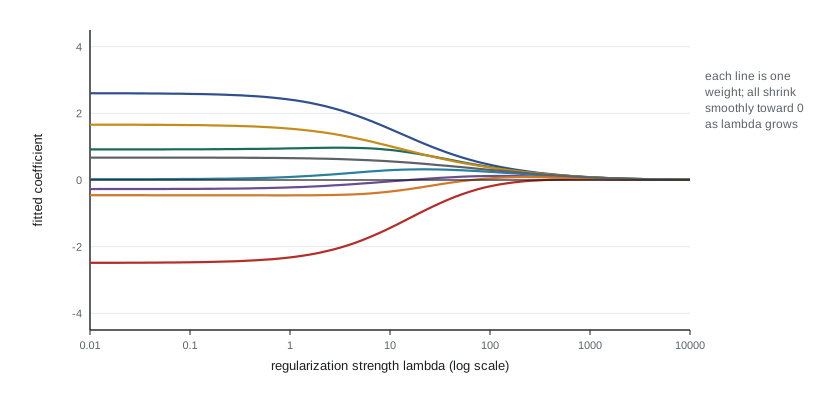
The regularization strength \(\lambda \ge 0\) controls the trade-off. At \(\lambda = 0\) ridge is least squares; as \(\lambda\) grows, the weights shrink toward zero and the model becomes simpler. Adding \(\lambda I\) also makes the matrix invertible for any \(\lambda > 0\), so ridge has a unique solution even with more features than examples. The intercept is conventionally left unpenalized (centre the features and target first), and features should be standardized, because the penalty treats all weights alike and a feature measured in millimetres would otherwise be penalized far more than the same feature in kilometres.

In bias–variance terms, ridge accepts a little bias in exchange for a large reduction in variance. In Bayesian terms, it is the maximum a posteriori (MAP) estimate under a Gaussian prior \(\mathbf{w} \sim \mathcal{N}(0, \tau^2 I)\) with \(\lambda = \sigma^2 / \tau^2\): the prior expresses a belief that large weights are unlikely. In terms of the singular value decomposition of X, ridge shrinks the component of the fit along each singular direction by the factor \(d_j^2 / (d_j^2 + \lambda)\), where \(d_j\) is the singular value, so it shrinks most strongly the poorly determined directions, which are exactly the ones that cause instability.

# Ridge regression on a small, collinear problem: choosing lambda on validation data.
import numpy as np
rng = np.random.default_rng(3)
n_tr, n_va, p = 40, 1000, 30
w_true = np.zeros(p); w_true[:5] = [3, -2, 1.5, 1, -1]     # only 5 features matter
def make(n):
    shared = rng.normal(size=(n, 1))               # a common factor makes all features correlated
    base = 0.8 * shared + 0.6 * rng.normal(size=(n, p))
    return base, base @ w_true + rng.normal(0, 2, n)
Xtr, ytr = make(n_tr); Xva, yva = make(n_va)

def ridge(X, y, lam):
    """Closed form: w = (X^T X + lam I)^(-1) X^T y (features have mean zero, no intercept)."""
    return np.linalg.solve(X.T @ X + lam * np.eye(X.shape[1]), X.T @ y)

print("  lambda   ||w||   train MSE   validation MSE")
for lam in (0.0, 0.1, 1, 10, 30, 100, 1000):
    w = ridge(Xtr, ytr, lam)
    tr = np.mean((Xtr @ w - ytr) ** 2); va = np.mean((Xva @ w - yva) ** 2)
    print(f"{lam:8g}  {np.linalg.norm(w):6.2f}  {tr:10.2f}  {va:15.2f}")

  lambda   ||w||   train MSE   validation MSE
       0   12.50        0.53            48.30
     0.1    9.60        0.59            26.85
       1    5.79        1.09             9.58
      10    2.45        3.31             6.47
      30    1.36        5.02             7.85
     100    0.71        6.71             9.23
    1000    0.29        9.77            10.38

With \(\lambda = 0\) the fit uses all 30 weights to chase noise in 40 examples: its training MSE is far below the noise variance of 4 and its validation MSE is about 48. Moderate regularization, around \(\lambda = 10\), cuts the validation error to about 6.5, a sevenfold improvement; very heavy regularization shrinks the weights so much that the model underfits and validation error rises again. The best \(\lambda\) has to be found from data, by validation or cross-validation (lesson 9), typically searching over a logarithmic grid such as 0.001, 0.01, ..., 1,000.

The lasso and sparsity

Robert Tibshirani's lasso (least absolute shrinkage and selection operator, 1996) replaces the squared penalty with the sum of absolute values, the \(\ell_1\) norm:

The change has a striking effect: the lasso sets many weights exactly to zero, so it performs feature selection as part of fitting. The geometric reason is that the \(\ell_1\) constraint region \(\lVert \mathbf{w} \rVert_1 \le t\) is a diamond (in two dimensions) or a cross-polytope with corners on the axes, and the elliptical contours of the squared loss usually touch it first at a corner, where some coordinates are zero. The \(\ell_2\) ball of ridge is round and has no corners. The lasso has no closed-form solution, because the absolute value is not differentiable at zero, but coordinate descent solves it efficiently: update one weight at a time, holding the others fixed, using the soft-thresholding operator \(S(z, t) = \mathrm{sign}(z) \max(\lvert z \rvert - t, 0)\).

# Lasso by coordinate descent with soft-thresholding: many weights become exactly zero.
import numpy as np
rng = np.random.default_rng(3)
n, p = 100, 30
w_true = np.zeros(p); w_true[:5] = [3, -2, 1.5, 1, -1]
X = rng.normal(size=(n, p)); y = X @ w_true + rng.normal(0, 1, n)

def soft(z, t):
    return np.sign(z) * max(abs(z) - t, 0.0)

def lasso(X, y, lam, sweeps=200):
    """Minimize (1/2n)||y - Xw||^2 + lam * ||w||_1 one coordinate at a time."""
    n, p = X.shape; w = np.zeros(p); col_sq = (X ** 2).sum(axis=0) / n
    for _ in range(sweeps):
        for j in range(p):
            r_j = y - X @ w + X[:, j] * w[j]           # residual ignoring feature j
            w[j] = soft(X[:, j] @ r_j / n, lam) / col_sq[j]
    return w

for lam in (0.01, 0.1, 0.3, 1.0):
    w = lasso(X, y, lam)
    nz = np.flatnonzero(np.abs(w) > 1e-10)
    print(f"lambda {lam:4}: {nz.size:2} nonzero weights; first five = {np.round(w[:5], 2)}")

lambda 0.01: 29 nonzero weights; first five = [ 2.98 -1.81  1.7   0.94 -1.03]
lambda  0.1: 14 nonzero weights; first five = [ 2.78 -1.76  1.48  0.88 -0.93]
lambda  0.3:  5 nonzero weights; first five = [ 2.53 -1.58  1.27  0.78 -0.74]
lambda  1.0:  5 nonzero weights; first five = [ 1.66 -0.99  0.58  0.32 -0.05]

With a small \(\lambda\) almost every weight is nonzero, though most are small; as \(\lambda\) increases, the irrelevant weights drop out, and at \(\lambda = 0.3\) the lasso keeps exactly the five features that matter, with their weights shrunk somewhat toward zero. At \(\lambda = 1\) the same five survive but are shrunk heavily (the fifth almost to zero), and a slightly larger value would start removing real features. The elastic net, which combines \(\ell_1\) and \(\ell_2\) penalties, keeps the lasso's sparsity while behaving better when features come in correlated groups, where the lasso tends to pick one member arbitrarily.

Practical notes

Several practical points apply to every linear model. Standardize features before regularizing, using means and standard deviations computed on the training data only, never on validation or test data (lesson 10 explains why). Encode categorical features with indicator (one-hot) variables, dropping one category if an unpenalized intercept is present, to avoid exact collinearity. Inspect residuals: a curved pattern suggests missing nonlinear features, a funnel shape suggests that the noise variance grows with the prediction and a log transform of the target may help. Watch for outliers, which squared loss weighs heavily. And remember that a regularized coefficient is a biased estimate; if the goal is to interpret coefficients or test hypotheses about them, the inferential tools of STAT-151 apply to unregularized fits, and post-selection inference after the lasso is a subtle topic of its own.

Linear regression is also the building block for more flexible methods. Kernel ridge regression (lesson 5) applies ridge in a high-dimensional feature space without computing the features. Gradient boosting (lesson 7) fits a sequence of simple models to residuals. And the last layer of most neural networks is a linear model on learned features.

Worked examples