Feature engineering, pipelines and practical machine learning

The algorithms of the previous lessons all start from a table of numbers. Real data arrive as something messier: customer records with missing fields, categories spelled three ways, dates, free text, measurements in different units, and rare events buried among common ones. Turning raw data into features a model can use, and doing so without fooling yourself, is where much of the work and much of the risk of a machine learning project lies. This lesson covers the core preprocessing steps, the pipeline discipline that keeps them honest, the many forms of data leakage, class imbalance, and the habits that make results reproducible. AI-220 treats data engineering at scale, and AI-420 treats deploying and monitoring models in production; here the focus is on the modelling workflow itself.

Numerical features: scaling and transformation

Many methods are sensitive to the scale of features: k-NN and RBF kernels through distances, regularized linear models through the penalty, gradient descent through conditioning. Standardization subtracts the mean and divides by the standard deviation; min–max scaling maps each feature to [0, 1]; robust scaling uses the median and interquartile range, which outliers cannot distort. Tree-based methods are indifferent to monotone transformations and need none of this.

Transformations can also make relationships easier to learn. Skewed positive quantities such as income, prices and counts often behave better on a logarithmic scale, where multiplicative effects become additive. Binning a continuous feature into intervals lets a linear model capture a non-monotone effect at the cost of resolution. Polynomial and interaction features (lesson 3) let linear models represent curvature and dependence between features. Domain knowledge supplies the best features of all: the ratio of debt to income says more than either alone; the time since a customer's last purchase says more than the date of the purchase.

Categorical features

A categorical feature such as province, product type or plan cannot be fed to most models as an integer code, because 1, 2, 3 imposes an order and spacing that do not exist. One-hot encoding replaces a feature with K categories by K indicator columns, exactly one of which is 1. For a linear model with an intercept, one column is redundant and is often dropped to avoid exact collinearity. High-cardinality categories, such as postal codes or product identifiers with thousands of values, make one-hot encoding unwieldy; alternatives include grouping rare categories into an other bucket, hashing categories into a fixed number of columns, learned embeddings, and target encoding, which replaces each category by the mean target among training examples in that category. Target encoding is powerful but leaks the target unless it is computed out of fold, the same subtlety that CatBoost's ordered statistics address.

Missing values

Missing data are the rule, not the exception. The first question is why values are missing. If they are missing completely at random, simple imputation is reasonable: replace with the training mean or median for numbers, or the most frequent value or a new missing category for categories. If missingness depends on other features, model-based imputation (predicting the missing value from the others, as in k-NN imputation or iterative imputation) is better. If missingness depends on the value itself, as when people with high incomes decline to report them, no imputation recovers the truth, and the fact of missingness can itself be informative: adding an indicator column that marks which values were imputed often helps. Some models, including gradient-boosted trees in XGBoost, LightGBM and scikit-learn's histogram-based estimators, handle missing values natively by learning which branch they should follow.

Text, dates and other raw data

Text can be turned into features with the bag-of-words counts of lesson 8, often reweighted by TF–IDF (term frequency times inverse document frequency) to downweight words that appear everywhere, and extended with word pairs (bigrams). Modern practice increasingly uses embeddings from pretrained language models, which AI-340 and AI-410 cover. Dates should be decomposed into features that matter for the problem: day of week, hour, month, whether a holiday, time since some event; cyclic features such as hour of day can be encoded with sine and cosine so that 23:00 is near 00:00. Images and audio are now almost always handled with deep networks (CMPUT-466, AI-350), though classical feature extraction still appears in constrained settings.

Pipelines: fit on training data only

Every preprocessing step that learns something from data (a mean for standardization, a median for imputation, a vocabulary, a set of selected features, a category encoding) is part of the model, and must be fitted on training data only. Computing the scaling statistics on the full data set before splitting lets information from the validation and test sets leak into training. For standardization the effect is usually small; for feature selection, target encoding or imputation it can be enormous. The program below shows the classic demonstration, due to Ambroise and McLachlan's 2002 critique of gene-expression studies: choosing features using all the data makes pure noise look predictive.

# Leakage by feature selection: choosing features on all the data before cross-validation.
import numpy as np
from sklearn.feature_selection import SelectKBest, f_classif
from sklearn.linear_model import LogisticRegression
from sklearn.model_selection import cross_val_score
from sklearn.pipeline import make_pipeline
rng = np.random.default_rng(367)
X = rng.normal(size=(100, 5000))          # 5,000 features of pure noise
y = rng.integers(0, 2, 100)               # labels unrelated to X: true accuracy is 50%

# wrong: pick the 20 features most correlated with y using ALL rows, then cross-validate
X_sel = SelectKBest(f_classif, k=20).fit_transform(X, y)
wrong = cross_val_score(LogisticRegression(max_iter=1000), X_sel, y, cv=5).mean()
# right: selection happens inside each training fold, as part of the pipeline
pipe = make_pipeline(SelectKBest(f_classif, k=20), LogisticRegression(max_iter=1000))
right = cross_val_score(pipe, X, y, cv=5).mean()
print(f"selection outside CV: estimated accuracy {wrong:.2f}")
print(f"selection inside CV:  estimated accuracy {right:.2f}")

selection outside CV: estimated accuracy 0.85
selection inside CV:  estimated accuracy 0.49

The labels are coin flips, so no model can do better than 50 per cent. Selecting the 20 features most correlated with the labels on all 100 examples, then cross-validating, reports an accuracy far above chance, because the selection step already saw the validation folds and picked features that happen to fit them. Putting selection inside the pipeline, so it is refitted on each training fold, gives an honest estimate near 50 per cent. Published studies have made exactly this mistake.

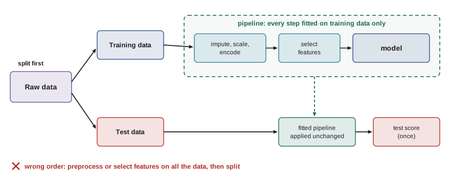
Scikit-learn's Pipeline and ColumnTransformer objects encode this discipline: the whole chain of preprocessing and model is a single estimator, so cross-validation and grid search refit every step on each training fold automatically. The next program builds a complete pipeline for an invented churn problem with numeric and categorical features, missing values, and a hyperparameter search.

# A full preprocessing and model pipeline on invented customer-churn data (Canada).
import numpy as np, pandas as pd
rng = np.random.default_rng(367)
n = 2000
region = rng.choice(["AB", "BC", "ON", "QC", "NS"], n, p=[0.15, 0.2, 0.35, 0.22, 0.08])
plan = rng.choice(["basic", "plus", "premium"], n)
tenure = rng.integers(1, 72, n).astype(float)               # months as a customer
monthly = np.round(rng.normal(60, 20, n), 2)
calls = rng.poisson(1.5, n).astype(float)                   # support calls last quarter
logit = -1.0 - 0.04 * tenure + 0.02 * (monthly - 60) + 0.5 * calls + 0.8 * (plan == "basic")
y = (rng.uniform(size=n) < 1 / (1 + np.exp(-logit))).astype(int)
monthly[rng.uniform(size=n) < 0.05] = np.nan                # 5% missing values
df = pd.DataFrame({"region": region, "plan": plan, "tenure": tenure, "monthly": monthly, "calls": calls})

from sklearn.compose import ColumnTransformer
from sklearn.pipeline import Pipeline
from sklearn.preprocessing import OneHotEncoder, StandardScaler
from sklearn.impute import SimpleImputer
from sklearn.linear_model import LogisticRegression
from sklearn.model_selection import train_test_split, GridSearchCV
prep = ColumnTransformer([
    ("num", Pipeline([("impute", SimpleImputer(strategy="median")), ("scale", StandardScaler())]),
     ["tenure", "monthly", "calls"]),
    ("cat", OneHotEncoder(handle_unknown="ignore"), ["region", "plan"])])
model = Pipeline([("prep", prep), ("clf", LogisticRegression(max_iter=1000))])
Xtr, Xte, ytr, yte = train_test_split(df, y, test_size=0.25, random_state=0, stratify=y)
search = GridSearchCV(model, {"clf__C": [0.01, 0.1, 1, 10]}, cv=5, scoring="roc_auc").fit(Xtr, ytr)
print(f"churn rate {y.mean():.3f}; best C = {search.best_params_['clf__C']}, CV AUC {search.best_score_:.3f}")
print(f"test AUC {search.score(Xte, yte):.3f}")
names = search.best_estimator_["prep"].get_feature_names_out()
coefs = search.best_estimator_["clf"].coef_[0]
for nm, c in sorted(zip(names, coefs), key=lambda t: -abs(t[1]))[:5]:
    print(f"   {nm:22} {c:+.3f}")

churn rate 0.248; best C = 0.1, CV AUC 0.765
test AUC 0.808
   num__tenure            -0.770
   num__calls             +0.534
   cat__plan_basic        +0.464
   cat__plan_premium      -0.336
   num__monthly           +0.330

The largest coefficients recover the drivers built into the invented data: tenure lowers churn risk, support calls raise it, and the basic plan raises it relative to the others, while the regions, which played no role in generating the labels, get small weights. Because every step lives inside the pipeline, the cross-validated AUC is an honest estimate for the tuning, and the test AUC, computed once, confirms it.

Other forms of leakage

Preprocessing is only one route by which information from outside the training data can contaminate a model. Shachar Kaufman and colleagues' 2012 survey and Sayash Kapoor and Arvind Narayanan's 2023 review of leakage across scientific fields catalogue many others. Target leakage occurs when a feature encodes the answer: a model predicting hospital readmission that uses a field recorded during the readmission, or a churn model using whether the customer has a cancellation fee on file. Temporal leakage occurs when a model is validated on the past using features computed from the future, such as a 30-day average that includes days after the prediction date. Group leakage occurs when near-duplicate examples, such as several images of one patient or one product photographed several times, straddle the split. A model that seems too good to be true usually is; the first suspect is leakage.

Class imbalance

In fraud detection, disease screening, equipment failure prediction and many other problems, the positive class is rare. Lesson 9 showed that accuracy is then misleading. Beyond choosing proper metrics, there are three families of remedy. First, change the decision threshold: a probabilistic model trained on imbalanced data predicts low probabilities for the rare class, which is correct, and the right threshold follows from the costs. Second, reweight the loss so that errors on the rare class count more; most scikit-learn classifiers accept a class_weight argument. Third, resample: undersample the majority class, oversample the minority class, or synthesize new minority examples with SMOTE (Chawla and colleagues, 2002), which interpolates between minority neighbours. Resampling must be done inside the training folds only, never before splitting.

# Class imbalance: class weights and threshold choice on invented data with 3% positives.
import numpy as np
from sklearn.linear_model import LogisticRegression
from sklearn.metrics import precision_score, recall_score
rng = np.random.default_rng(5)
def make(n):
    y = (rng.uniform(size=n) < 0.03).astype(int)
    X = rng.normal(size=(n, 4)) + y[:, None] * np.array([1.2, 0.8, 0.0, 0.5])
    return X, y
Xtr, ytr = make(6000); Xte, yte = make(20000)
for name, m in [("unweighted", LogisticRegression()), ("class_weight='balanced'", LogisticRegression(class_weight="balanced"))]:
    p = m.fit(Xtr, ytr).predict_proba(Xte)[:, 1]
    for t in (0.5, 0.1):
        pred = (p >= t).astype(int)
        print(f"{name:24} threshold {t}: recall {recall_score(yte, pred):.3f}, "
              f"precision {precision_score(yte, pred, zero_division=0):.3f}, mean P(positive) {p.mean():.3f}")

unweighted               threshold 0.5: recall 0.063, precision 0.609, mean P(positive) 0.032
unweighted               threshold 0.1: recall 0.470, precision 0.200, mean P(positive) 0.032
class_weight='balanced'  threshold 0.5: recall 0.755, precision 0.106, mean P(positive) 0.307
class_weight='balanced'  threshold 0.1: recall 0.973, precision 0.045, mean P(positive) 0.307

With the default threshold of 0.5, the unweighted model rarely predicts the rare class at all. Lowering its threshold to 0.1 recovers much of the recall, at a cost in precision. Class weighting has a similar effect at the default threshold, by inflating the predicted probabilities: the weighted model's mean predicted probability is far above the true positive rate of 3 per cent, so its probabilities are no longer calibrated. That is often acceptable if only the ranking or a decision matters, but if calibrated probabilities are needed, prefer threshold adjustment or recalibrate afterward.

Hyperparameter search

Most models have hyperparameters: λ for ridge, C and γ for SVMs, k for k-NN, depth and learning rate for boosting. Grid search tries every combination on a grid and is fine for one or two hyperparameters. Random search, which James Bergstra and Yoshua Bengio showed in 2012 is usually more efficient, samples combinations at random, so that with several hyperparameters of which only a few matter, it explores many more distinct values of the important ones. Bayesian optimization builds a model of validation error as a function of the hyperparameters and chooses the next trial to balance exploration and exploitation; AI-310 covers it. Search over logarithmic scales for scale parameters such as λ, C, γ and learning rates, and keep the search inside the training data with cross-validation.

Reproducibility

A result that cannot be reproduced cannot be trusted or improved. Fix random seeds for data splits, model initialization and resampling, and record them. Record library versions, since default settings change between releases. Keep the code that produced every number, from raw data to final table, under version control; notebooks are convenient for exploration but are easily run out of order. Save the exact training, validation and test splits. Report the variation across seeds rather than the best run. These habits, which AI-110 and AI-420 develop, cost little and save weeks when a result must be explained, extended or corrected months later.

From validation to the real world

A model that performs well on a held-out test set can still fail after deployment, because the deployment distribution differs from the training distribution: covariate shift (the inputs change, as when a new customer segment arrives), label or prior shift (the base rate changes), or concept drift (the relationship between inputs and outputs changes, as when fraudsters adapt). Feedback loops make matters worse: a model that decides who receives a loan determines which outcomes are ever observed. Monitoring input distributions, prediction distributions and, when labels arrive, performance over time is part of the job, and AI-420 covers it in detail. The formal setup of lesson 1 assumes a fixed distribution; practice requires checking that assumption continually.

Worked examples