Dimensionality reduction, neural networks and a capstone project

This final lesson completes the toolkit and puts it to work. It begins with principal component analysis, the most important method for reducing the dimension of data, which compresses many correlated features into a few informative ones and counters the curse of dimensionality of lesson 6. It then takes a first step beyond the linear and tree-based models of this course to a small neural network, trained by backpropagation, as a bridge to CMPUT-466. It closes with a capstone that runs a complete supervised learning project, from framing to a check of how the chosen model treats different groups, and with a short survey of the responsibilities that come with deploying machine learning.

Principal component analysis

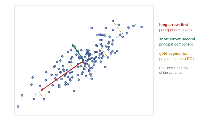
Data in many dimensions often vary mostly along a few directions. Measurements of the height, arm span and leg length of people are strongly correlated and mostly reflect overall size; the 64 pixels of a small image of a handwritten digit are far from independent. Principal component analysis (PCA), introduced by Karl Pearson in 1901 and developed by Harold Hotelling in 1933, finds an orthogonal set of directions ordered by how much of the data's variance lies along each. Projecting onto the first k directions gives the best k-dimensional linear summary of the data.

Two derivations lead to the same answer. First, maximum variance: centre the data (subtract each feature's mean) and look for the unit vector \(\mathbf{v}\) maximizing the variance of the projections \(\mathbf{v}^{\top}\mathbf{x}_i\), which is \(\mathbf{v}^{\top} C \mathbf{v}\) with C the sample covariance matrix. With a Lagrange multiplier for the constraint \(\lVert \mathbf{v} \rVert = 1\), the stationarity condition is

so the best direction is the eigenvector of C with the largest eigenvalue, and the variance captured is that eigenvalue. The second principal component is the best direction orthogonal to the first, which is the eigenvector with the second-largest eigenvalue, and so on. Second, minimum reconstruction error: among all k-dimensional linear subspaces, the span of the top k eigenvectors minimizes the mean squared distance between the points and their projections. The two views agree because, for centred data, total variance equals variance captured plus reconstruction error.

In practice PCA is computed with the singular value decomposition of the centred data matrix, \(X_c = U S V^{\top}\), which is more accurate than forming C. The rows of \(V^{\top}\) are the principal directions, the projections are \(X_c V_k\), and the variance along direction j is \(s_j^2/(n-1)\). For very large data, randomized SVD or power iteration (repeatedly multiplying a vector by C and normalizing) find the leading components without a full decomposition. AI-210 develops the SVD in depth.

# Principal component analysis from scratch with the SVD, on scikit-learn's bundled 8x8 digit images.
import numpy as np
from sklearn.datasets import load_digits
X = load_digits().data                         # 1,797 images, 64 pixel features each
Xc = X - X.mean(axis=0)                        # subtract each feature's mean
U, S, Vt = np.linalg.svd(Xc, full_matrices=False)
var = S ** 2 / (len(X) - 1)                    # variance along each principal direction
ratio = np.cumsum(var) / var.sum()
for k in (1, 2, 5, 10, 20, 30, 40):
    Z = Xc @ Vt[:k].T                          # project onto the first k components
    recon = Z @ Vt[:k]                         # map back to 64 dimensions
    err = np.mean((Xc - recon) ** 2)
    print(f"k = {k:2}: cumulative variance explained {ratio[k - 1]:.3f}, mean squared reconstruction error {err:6.2f}")
print("components needed for 90% of the variance:", int(np.searchsorted(ratio, 0.90) + 1))

# power iteration finds the first principal direction without a full SVD
v = np.ones(64) / 8; C = Xc.T @ Xc / (len(X) - 1)
for _ in range(200):
    v = C @ v; v /= np.linalg.norm(v)
print(f"power iteration: |cosine with first SVD direction| = {abs(v @ Vt[0]):.6f}, eigenvalue {v @ C @ v:.2f} vs {var[0]:.2f}")

k =  1: cumulative variance explained 0.149, mean squared reconstruction error  15.98
k =  2: cumulative variance explained 0.285, mean squared reconstruction error  13.42
k =  5: cumulative variance explained 0.545, mean squared reconstruction error   8.54
k = 10: cumulative variance explained 0.738, mean squared reconstruction error   4.91
k = 20: cumulative variance explained 0.894, mean squared reconstruction error   1.98
k = 30: cumulative variance explained 0.959, mean squared reconstruction error   0.77
k = 40: cumulative variance explained 0.988, mean squared reconstruction error   0.22
components needed for 90% of the variance: 21
power iteration: |cosine with first SVD direction| = 1.000000, eigenvalue 179.01 vs 179.01

The digit images live in 64 dimensions, but about 20 components capture 90 per cent of their variance, and reconstruction error falls steeply over the first few components and slowly after that. Power iteration recovers the first direction essentially exactly. A plot of cumulative explained variance against k, called a scree plot, is the usual guide for choosing k, alongside the performance of whatever task the reduced data serve.

Using PCA well

PCA has several uses: visualization (project to two or three dimensions and plot), compression, noise reduction (discard the low-variance components, which often contain mostly noise), decorrelating features before methods that dislike collinearity, and speeding up downstream learning. Used as preprocessing, it must sit inside the pipeline, fitted on training data only, like any other learned step. Standardize first if features are in different units, or PCA will simply find the feature with the largest numbers.

# PCA as preprocessing: accuracy of logistic regression on the digits with k components.
import numpy as np
from sklearn.datasets import load_digits
from sklearn.decomposition import PCA
from sklearn.linear_model import LogisticRegression
from sklearn.model_selection import cross_val_score
from sklearn.pipeline import make_pipeline
from sklearn.preprocessing import StandardScaler
X, y = load_digits(return_X_y=True)
for k in (2, 5, 10, 20, 40, 64):
    pipe = make_pipeline(StandardScaler(), PCA(n_components=k), LogisticRegression(max_iter=5000))
    print(f"{k:2} components: 5-fold CV accuracy {cross_val_score(pipe, X, y, cv=5).mean():.3f}")

 2 components: 5-fold CV accuracy 0.535
 5 components: 5-fold CV accuracy 0.771
10 components: 5-fold CV accuracy 0.840
20 components: 5-fold CV accuracy 0.899
40 components: 5-fold CV accuracy 0.914
64 components: 5-fold CV accuracy 0.920

PCA is unsupervised: it keeps the directions of greatest variance, which need not be the directions that matter for prediction. A small-variance direction may carry all the class information, and LDA (lesson 8) or simply regularized models on the full features may then do better. PCA is also linear. Nonlinear methods for visualization, notably t-SNE (Laurens van der Maaten and Geoffrey Hinton, 2008) and UMAP (Leland McInnes and colleagues, 2018), place points so that neighbours in the original space stay neighbours in two dimensions, and often reveal cluster structure that PCA blurs. Their plots must be read with care: distances between clusters and cluster sizes are not meaningful, results change with the perplexity or neighbourhood parameter and the random seed, and apparent clusters can appear in structureless data. Use them to explore, not to prove. Autoencoders, neural networks trained to reconstruct their input through a narrow middle layer, are the nonlinear generalization of PCA that CMPUT-466 covers.

A first neural network

Lesson 4 noted that a single linear unit cannot compute exclusive or. A network with one hidden layer can. Each hidden unit computes a linear function of the inputs followed by a nonlinearity such as tanh or the rectified linear unit \(\max(0, z)\); the output unit is a logistic regression on the hidden units' outputs. The hidden layer learns its own features, transforming the inputs into a representation in which the classes are linearly separable. With enough hidden units, such a network can approximate any continuous function on a bounded region, the universal approximation theorem of George Cybenko (1989) and Kurt Hornik (1991), though the theorem says nothing about how many units are needed or whether training will find them.

Training uses gradient descent on the cross-entropy loss, and the gradients are computed by backpropagation: an application of the chain rule that passes error signals backward from the output through each layer, reusing intermediate results so that the cost of computing all gradients is about the same as one forward pass. The idea was discovered several times; its 1986 popularization by David Rumelhart, Geoffrey Hinton and Ronald Williams revived neural network research. Hinton, who spent much of his career at the University of Toronto, shared the 2018 Turing Award with Yoshua Bengio of Université de Montréal and Yann LeCun for deep learning, and shared the 2024 Nobel Prize in Physics with John Hopfield.

# A two-layer neural network learns exclusive or by backpropagation, written from scratch.
import numpy as np
rng = np.random.default_rng(367)
X = np.array([[0, 0], [0, 1], [1, 0], [1, 1]], dtype=float)
y = np.array([[0], [1], [1], [0]], dtype=float)        # XOR: no single line separates the classes

W1 = rng.normal(0, 1, (2, 4)); b1 = np.zeros(4)         # 4 hidden units
W2 = rng.normal(0, 1, (4, 1)); b2 = np.zeros(1)
sig = lambda z: 1 / (1 + np.exp(-z))
lr = 1.0
for step in range(1, 5001):
    H = np.tanh(X @ W1 + b1)                            # forward pass: hidden layer
    p = sig(H @ W2 + b2)                                # output probability
    loss = -np.mean(y * np.log(p) + (1 - y) * np.log(1 - p))
    d_out = (p - y) / len(X)                            # backward pass: gradient at the output score
    dW2 = H.T @ d_out; db2 = d_out.sum(axis=0)
    d_hid = (d_out @ W2.T) * (1 - H ** 2)               # chain rule through tanh
    dW1 = X.T @ d_hid; db1 = d_hid.sum(axis=0)
    W1 -= lr * dW1; b1 -= lr * db1; W2 -= lr * dW2; b2 -= lr * db2
    if step in (1, 100, 1000, 5000):
        print(f"step {step:4}: loss {loss:.4f}   predictions {np.round(p.ravel(), 3)}")

step    1: loss 0.7719   predictions [0.5   0.83  0.66  0.833]
step  100: loss 0.0328   predictions [0.007 0.964 0.966 0.051]
step 1000: loss 0.0025   predictions [0.    0.997 0.997 0.004]
step 5000: loss 0.0005   predictions [0.    0.999 0.999 0.001]

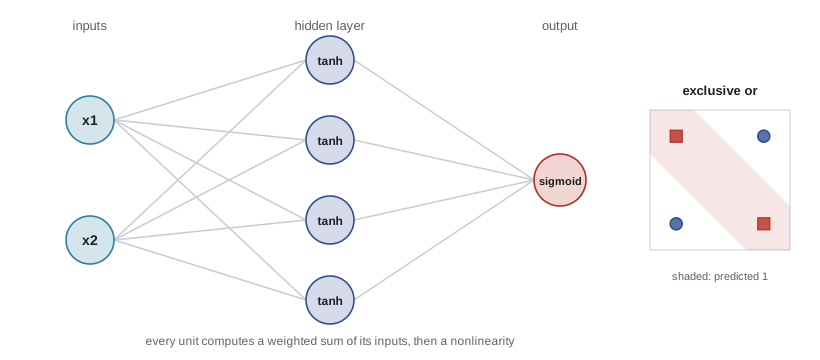
The loss falls and the four predictions approach their targets. Even this tiny example shows features that distinguish neural network training from the convex problems earlier in the course: the loss is not convex, the result depends on the random initialization, and the learning rate matters. Scaling these ideas to millions of parameters, with convolutional and attention layers, careful initialization, normalization, adaptive optimizers and regularization methods such as dropout, is the subject of CMPUT-466 and AI-410. Everything in this course still applies: the bias–variance trade-off, held-out evaluation, leakage and calibration are as important for a billion-parameter model as for a ridge regression, though very large networks show behaviours, such as double descent, that classical theory did not anticipate.

Capstone: an end-to-end project

The capstone brings the course together on an invented problem: predicting whether a personal loan will be repaid, using four features available at application time, namely income, debt ratio, years of credit history and recent late payments. The data also record an invented demographic attribute, called group here, which is deliberately not used as a feature but is retained so that the model's behaviour can be checked across groups. The steps follow lesson 1's project outline. The problem is binary classification with costly errors in both directions: a default loses money, and a wrongful refusal harms an applicant who would have repaid. Data are split once, with a stratified 25 per cent test set held back. Three model families are compared by five-fold cross-validated AUC on the training data: a regularized logistic regression inside a scaling pipeline, a random forest and gradient-boosted trees. The one with the best cross-validated AUC is fitted on all the training data and evaluated once on the test set. Finally, approval decisions at a threshold are examined separately for each group.

# Capstone: comparing three model families on invented loan-repayment data, then a test-set and subgroup check.
import numpy as np
from sklearn.linear_model import LogisticRegression
from sklearn.ensemble import RandomForestClassifier, GradientBoostingClassifier
from sklearn.model_selection import cross_val_score, train_test_split
from sklearn.pipeline import make_pipeline
from sklearn.preprocessing import StandardScaler
from sklearn.metrics import roc_auc_score
rng = np.random.default_rng(367)
n = 4000
group = rng.integers(0, 2, n)                        # an invented demographic attribute, NOT used as a feature
income = rng.lognormal(10.8 - 0.15 * group, 0.4, n) / 1000          # thousands
debt_ratio = np.clip(rng.normal(0.35 + 0.03 * group, 0.12, n), 0, 1)
history = rng.integers(0, 25, n)                    # years of credit history
late = rng.poisson(0.6 + 0.8 * debt_ratio, n)       # late payments in the past two years
logit = 1.5 + 0.02 * (income - 50) - 4 * (debt_ratio - 0.35) + 0.05 * history - 0.7 * late - 0.6 * (debt_ratio > 0.5) * late
y = (rng.uniform(size=n) < 1 / (1 + np.exp(-logit))).astype(int)    # 1 = repaid
X = np.column_stack([income, debt_ratio, history, late])
Xtr, Xte, ytr, yte, gtr, gte = train_test_split(X, y, group, test_size=0.25, random_state=0, stratify=y)

models = {"logistic regression": make_pipeline(StandardScaler(), LogisticRegression()),
          "random forest": RandomForestClassifier(n_estimators=300, min_samples_leaf=5, random_state=0),
          "gradient boosting": GradientBoostingClassifier(n_estimators=200, learning_rate=0.05, max_depth=3, random_state=0)}
cv = {}
for name, m in models.items():
    s = cross_val_score(m, Xtr, ytr, cv=5, scoring="roc_auc"); cv[name] = s.mean()
    print(f"{name:20} 5-fold CV AUC {s.mean():.3f} ± {s.std() / np.sqrt(5):.3f}")
choice = max(cv, key=cv.get)                       # choose by cross-validation, never by test score
p = models[choice].fit(Xtr, ytr).predict_proba(Xte)[:, 1]
print(f"chosen model: {choice}; test AUC {roc_auc_score(yte, p):.3f} (evaluated once)")
approve = p >= 0.7
for g in (0, 1):
    m = gte == g
    tpr = approve[m & (yte == 1)].mean()
    print(f"group {g}: approval rate {approve[m].mean():.3f}, approval rate among those who repay {tpr:.3f}, test AUC {roc_auc_score(yte[m], p[m]):.3f}")

logistic regression  5-fold CV AUC 0.779 ± 0.008
random forest        5-fold CV AUC 0.753 ± 0.008
gradient boosting    5-fold CV AUC 0.768 ± 0.007
chosen model: logistic regression; test AUC 0.766 (evaluated once)
group 0: approval rate 0.729, approval rate among those who repay 0.804, test AUC 0.737
group 1: approval rate 0.618, approval rate among those who repay 0.732, test AUC 0.787

Logistic regression wins the cross-validated comparison, ahead of gradient boosting by a little more than one standard error and of the random forest by about three, even though the data contain an interaction (late payments matter more when the debt ratio is high) that the tree ensembles could in principle capture and the linear model cannot. With four features, a smooth relationship and a few thousand examples, the linear model's low variance outweighs its small bias, while the ensembles, at these settings, spend their flexibility partly on noise. That outcome is common on modest tabular data, and it is a useful corrective to the reputation of ensembles: always include a well-regularized linear baseline. The chosen model's test AUC, computed once, agrees with its cross-validation estimate. A linear model also has practical advantages here, since lenders must be able to give applicants the principal reasons for a refusal.

The subgroup check is the step most often skipped. The group attribute was never given to the model, yet the approval rates differ, because income and debt ratio differ between the groups in the invented data. At a threshold of 0.7, group 1's approval rate is about 11 points lower than group 0's, and among applicants who in fact repaid, group 1 members were refused more often (27 per cent against 20 per cent). Whether that difference is acceptable is not a statistical question. Several fairness criteria can be measured: demographic parity compares approval rates; equal opportunity compares approval rates among applicants who would repay (true positive rates); calibration within groups asks whether a predicted probability means the same thing in each group. Results by Jon Kleinberg, Sendhil Mullainathan and Manish Raghavan and by Alexandra Chouldechova (both 2016–2017) show that when base rates differ, these criteria generally cannot all hold at once, so choosing among them is a value judgement that the people affected and the law must inform. AI-460 develops these measures and the methods for mitigating unfair outcomes; the point here is that checking them is part of evaluating a model, not an optional extra.

Responsible machine learning

A deployed model makes or shapes decisions about people, and the habits of this course are the foundation of using it responsibly: honest evaluation on data like the deployment population, attention to leakage and drift, calibrated probabilities where decisions use them, and reporting performance by subgroup. Documentation such as model cards and datasheets records intended use and known limitations. Privacy matters too: models can memorize and leak training data, and AI-460 covers differential privacy and related defences.

In Canada, the proposed Artificial Intelligence and Data Act (AIDA), part of Bill C-27, would have regulated high-impact AI systems, but it died on the order paper when Parliament was prorogued in January 2025. In June 2026 the federal government released a national AI strategy, 'AI for All', that emphasizes trust, AI literacy and commercialization rather than a general AI statute. On June 15, 2026 it introduced Bill C-36, which would replace the privacy provisions of PIPEDA with a Protecting Privacy and Consumer Data Act; among other things it would require organizations using automated decision systems for decisions with significant effects to describe that use and, on request, explain a specific prediction or decision. As of October 2026 the bill had not been passed. Quebec's Law 25 already requires organizations to inform people when a decision about them is made exclusively by automated processing. Check the current state of these rules before relying on this summary.

Rules change quickly, and no course can be a substitute for current legal advice. What does not change is the professional responsibility of the person who builds a model to know what it does, how well it does it, and for whom it fails.

Where to go next

This course has covered the classical core: the learning problem and generalization, linear and kernel methods, trees and ensembles, probabilistic classifiers, evaluation, practical workflow, clustering and dimensionality reduction. CMPUT-466 continues with deep learning. In the AI program, AI-310 deepens the optimization, AI-320 the probabilistic modelling, AI-330 adds reinforcement learning, AI-340 and AI-350 apply learning to language and vision, AI-420 covers production systems, and AI-460 covers fairness and privacy. The best way to consolidate the material is to take a real data set from a domain you care about and carry it through every step of the capstone yourself.

Worked examples