Traffic studies and data analysis

Every analysis in this course starts from data: how many vehicles, how fast, where they go, when and how often they crash. Sofia's first assignment on the Ridgeway Road study is to plan the data collection: which counts to take, where to put the radar, how many vehicles to measure, how to turn a two-day count into an annual average, and how to tell whether the speed problem residents complain about is real. This lesson covers the main traffic studies and the statistics used to interpret them.

Volume counts

Traffic volumes are collected in several ways. Permanent count stations, usually inductive loops or other in-pavement or roadside sensors, record volumes continuously at a small number of sites and provide the factors used to adjust short counts. Coverage counts, typically 24 or 48 hours with pneumatic tubes or temporary radar sensors, are taken at many sites on a rotating schedule. Turning movement counts at intersections record how many vehicles make each movement, usually in 15-minute intervals over the peak periods, by observers, video analytics or the signal system's own detectors.

Modern data sources add to these. Signal controllers log detector actuations; connected vehicle and smartphone data give travel times and speeds over whole networks; video analytics classify vehicles and count pedestrians and cyclists. Each source has biases. Probe data over-represent some vehicle types and trip purposes; automated counters can miss motorcycles or double-count trucks; video can struggle in snow and darkness. A careful study cross-checks sources and reports their limitations.

Counts are classified by vehicle type because trucks and buses affect capacity, pavement wear and safety differently from cars. Many agencies use a 13-class scheme based on axle counts and spacing. Pedestrian and cyclist counts, once rare, are now routine on urban corridors; they are needed to time crossings, to justify facilities, and to compute exposure for safety analysis.

From a short count to AADT

A 48-hour count in October does not directly give the annual average daily traffic. Traffic varies by month (higher in summer on recreational roads, lower in winter), by day of the week (lower on weekends on commuter routes), and by hour. Agencies derive adjustment factors from their permanent stations, grouped by road type. A short count is converted to AADT by dividing out the day-of-week and month effects:

where \(V_{24}\) is the average daily volume of the count, \(DOW\) the day-of-week factor (the ratio of that weekday's average to the annual daily average) and \(MF\) the monthly factor (the ratio of AADT to the average daily traffic in the month of the count). Agencies define their factors in different ways, multiplicative or divisive, so the definitions must be read carefully. An axle correction factor is also applied when the counter counts axle hits instead of vehicles.

Peak-hour analysis needs the variation within the hour as well. The peak hour factor (PHF) compares the hourly volume with four times the busiest 15-minute volume in that hour:

A PHF of 1.0 means the hour is perfectly uniform; values of 0.85 to 0.95 are typical on urban arterials, and lower values occur near schools, factories or stadiums where traffic arrives in a burst. Capacity analyses divide the hourly volume by the PHF to get the flow rate in the peak 15 minutes, because a facility that can carry the average flow of the hour may still overflow in its worst quarter hour.

Spot speed studies

A spot speed study measures the speeds of vehicles passing a point, usually with radar, lidar or a pair of detectors. It is used to set speed limits, to evaluate complaints, to check whether a traffic calming measure worked, and to select design speeds. To represent free-flowing traffic, the measurement site should be away from intersections and driveways, the observer or equipment should be inconspicuous, and only vehicles that are not closely following another (often those with headways of at least 4 or 5 seconds) should be recorded.

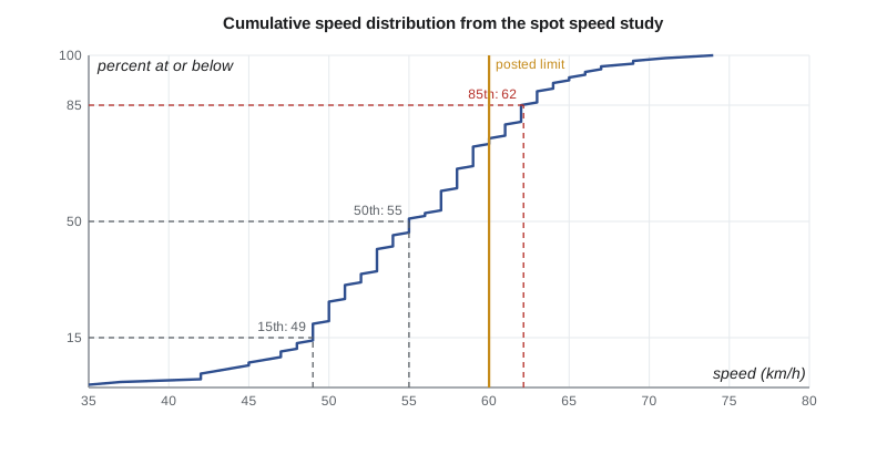
The results are summarized by the mean, the standard deviation and percentiles. The 85th percentile speed, the speed at or below which 85 % of vehicles travel, has long been used as a starting point for setting speed limits, on the theory that most drivers choose a reasonable speed. Current guidance in both countries treats it as only one input: the speed limit setting methods now in use also consider the road's context, the presence of people walking and cycling, crash history and the safe system principle that impact speeds should be kept within what the human body can tolerate. The pace, the range of a set width (often 15 km/h or 10 mph) containing the most vehicles, describes how uniform speeds are.

How many vehicles to measure

A sample of spot speeds estimates the true mean with an error that shrinks as the sample grows. If the standard deviation of speeds is \(s\) and we want the estimated mean to be within \(\pm E\) of the true mean at a confidence level corresponding to the normal deviate \(z\) (1.96 for 95 %), the required sample size is

With a standard deviation of 7 km/h, estimating the mean to within ±1.5 km/h at 95 % confidence needs about 84 vehicles. Estimating a percentile such as the 85th needs a larger sample, because percentiles are estimated less precisely than means. Many agencies require at least 100 vehicles per direction.

The Ridgeway Road speed study

Residents near the high school have complained that drivers on Ridgeway Road speed. The posted limit is 60 km/h. Sofia sets up a radar unit in an unmarked car mid-block, between Carrick Street and the school, on a dry weekday between 10 a.m. and noon, and records 120 free-flowing vehicles. A 48-hour tube count taken the same week totals 39,200 vehicles. The script summarizes the speeds, finds the pace, checks the sample size, and expands the count to AADT using the city's factors for October weekdays.

# Spot speed study on Ridgeway Road and expanding a short count
import random, statistics, math
UNITS = "SI"
SI = UNITS == "SI"
random.seed(390)
mean_true, sd_true = (56.0, 7.5) if SI else (34.5, 4.7)
speeds = sorted(round(random.gauss(mean_true, sd_true)) for _ in range(120))
n = len(speeds)
m = statistics.mean(speeds); s = statistics.stdev(speeds)
def pct(p):
    i = p / 100 * (n - 1); lo = int(i); f = i - lo
    return speeds[lo] + f * (speeds[min(lo + 1, n - 1)] - speeds[lo])
u = "km/h" if SI else "mph"
print(f"n = {n}, mean = {m:.1f} {u}, std dev = {s:.1f} {u}")
print(f"15th = {pct(15):.0f}, 50th = {pct(50):.0f}, 85th = {pct(85):.0f} {u}")
w = 15 if SI else 10
best = max(range(min(speeds), max(speeds) - w + 1), key=lambda a: sum(a <= x <= a + w for x in speeds))
print(f"{w} {u} pace: {best} to {best + w} {u} ({sum(best <= x <= best + w for x in speeds)/n*100:.0f} % of vehicles)")
E = 1.5 if SI else 1.0
need = (1.96 * s / E) ** 2
print(f"sample for +/- {E} {u} on the mean at 95 %: {math.ceil(need)} vehicles")
lim = 60 if SI else 35
print(f"share above the {lim} {u} limit: {sum(x > lim for x in speeds)/n*100:.0f} %")
# expand a 48-hour October weekday count to AADT
count48 = 39200          # vehicles in 48 h
dof = 1.04               # day-of-week factor (weekday counts run slightly high)
mof = 0.96               # monthly factor for October
aadt = count48 / 2 / dof * mof
print(f"AADT estimate = {aadt:,.0f} veh/d")
q15 = [412, 448, 495, 461]   # peak-hour 15-minute counts, both directions
phf = sum(q15) / (4 * max(q15))
print(f"peak hour = {sum(q15)} veh/h, PHF = {phf:.2f}")

n = 120, mean = 55.4 km/h, std dev = 7.0 km/h
15th = 49, 50th = 55, 85th = 62 km/h
15 km/h pace: 48 to 63 km/h (78 % of vehicles)
sample for +/- 1.5 km/h on the mean at 95 %: 85 vehicles
share above the 60 km/h limit: 25 %
AADT estimate = 18,092 veh/d
peak hour = 1816 veh/h, PHF = 0.92

The mean speed is about 55 km/h with a standard deviation of 7 km/h, and the 85th percentile is about 62 km/h, slightly above the 60 km/h limit; about a quarter of free-flowing drivers exceed the limit. The 120-vehicle sample is more than the 85 needed for the mean. The complaint is partly borne out: most drivers travel near the limit, but a substantial minority are faster, and 60 km/h is itself a high speed for a street where students cross. The AADT estimate of about 18,100 veh/d agrees well with the city's 2026 program value of 18,500, and the peak hour factor of 0.92 is typical of an arterial. These values feed lessons 6 and 10.

Comparing before and after

Traffic studies often ask whether something changed: did speeds fall after a road diet, did delay drop after retiming? Because of random variation, a difference in sample means is not proof of a real change. A standard test compares two means with the statistic

If \(|z|\) exceeds 1.96, the difference is significant at the 5 % level. For proportions, such as the share of drivers over the limit, a similar test uses the binomial variance. Statistical significance is not the same as practical importance: a speed reduction of 0.5 km/h (0.3 mph) may be statistically significant with a big sample and still be meaningless for safety.

Travel time, delay and origin-destination studies

Travel time studies measure how long it takes to traverse a corridor and where the delay occurs. The classic method is the floating car, in which a test vehicle drives the corridor several times, trying to pass as many vehicles as pass it, while recording the time at checkpoints. Today, probe vehicle data and Bluetooth or Wi-Fi readers that match device identifiers at two points give travel times continuously. Intersection delay studies count stopped vehicles at fixed intervals or measure control delay directly from video.

Origin-destination studies tell planners where trips start and end. Methods include roadside interviews, licence plate matching, household travel surveys and anonymized mobile device data. For the Ridgeway study, the team buys a sample of anonymized trip data and learns that about a third of the eastbound peak traffic past Carrick Street continues to the highway, using Ridgeway as a shortcut between the north end and the bypass. That finding becomes important in lesson 12, because through traffic can divert if the corridor changes.

Data quality, equipment and privacy

Field data are only as good as the way they were collected. Pneumatic tubes can be torn by plows or misread when vehicles stop on them; radar measures the cosine of the angle to the vehicle, so a unit set at a sharp angle reads low; video counts degrade in heavy snow, rain and low sun. A good study plan therefore includes a quality check: comparing the two directions of a count for plausibility, checking a sample of video counts by hand, confirming that the equipment's clock is right and that no holiday or event distorted the counting day. The study report states the dates, the weather, the equipment and any data rejected, so that someone reviewing it later can judge its reliability. Data that identify individuals, such as licence plates or device identifiers, must be handled under the privacy rules that apply to the agency: collected only for a stated purpose, anonymized or hashed as soon as possible, and deleted when no longer needed.

Crash data

Collision records come from police reports, compiled by provincial ministries into databases that municipalities can query. Reports record the location, time, conditions, vehicles, people and injury severity. They are invaluable but imperfect: many property-damage collisions go unreported, especially where drivers report them only at collision reporting centres, injury severity is judged at the scene, and locations can be coded inaccurately. Lesson 11 explains how statistical methods deal with the randomness of crash counts and the regression to the mean that makes a site with one bad year look dangerous.