Two-dimensional seepage and flow nets

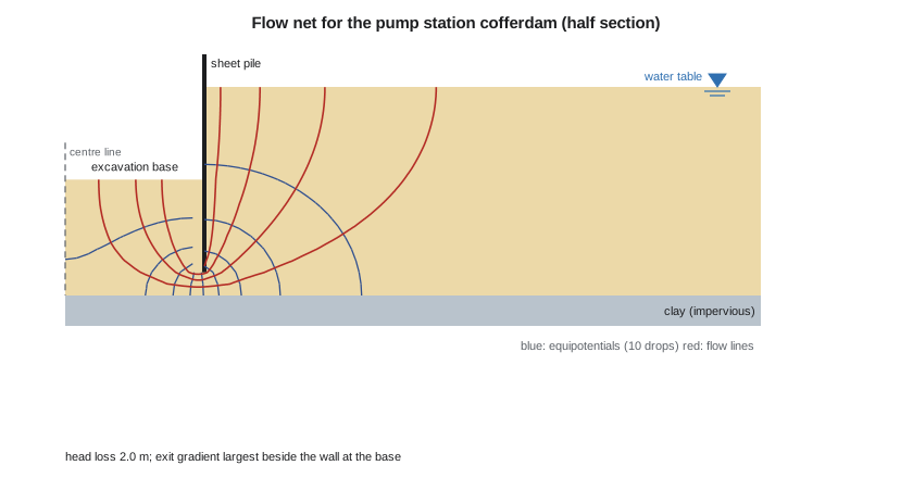
Most real seepage problems are not one-dimensional. Water flows under a dam, around the toe of a sheet pile wall and up into an excavation along curved paths, and the head and gradient vary from point to point. This lesson derives the equation that governs steady two-dimensional flow, shows how to solve it graphically with a flow net and numerically with a short program, and applies both to the sheet pile cofferdam for the new pump station at the operations centre. The answers needed are the inflow that the pumps must handle, the exit gradient against boiling and the safety of the clay at the base against uplift.

The pump station

The stormwater pump station sits at the north end of the site, where borehole BH-4 found the sand thicker than at the garage: sand from the surface to 7.0 m, grey clay from 7.0 to 12.0 m and till below. The water table is at 2.5 m, and a piezometer in the till reads 1.5 m below ground, as at BH-3. The wet well needs an excavation 6 m wide to 4.5 m depth. The contractor proposes steel sheet piles driven to 6.5 m, 2.0 m below the base, with pumps in a sump inside to keep the base dry.

Laplace's equation

Consider a small element of soil in a vertical plane, with flow in the x and z directions. If the soil is saturated and neither it nor the water compresses, as much water must leave the element as enters it. Combining this continuity condition with Darcy's law in each direction gives

For an isotropic soil, with \(k_x = k_z\), this becomes Laplace's equation, the same equation that governs steady heat conduction, electric potential and the flow of an ideal fluid:

The equation says nothing about the soil's permeability: the pattern of head depends only on the geometry and the boundary conditions. Permeability enters only when the flow rate is computed. Solving the equation means finding the head everywhere in the flow region, from which pore pressures, gradients and flows follow.

Boundary conditions

Every seepage problem has two kinds of boundary. On an equipotential boundary the total head is known and constant, such as the bed of a reservoir or the base of an excavation kept drained by pumps. On a no-flow boundary water cannot cross, so the gradient normal to the boundary is zero: an impermeable layer, the surface of a sheet pile or concrete dam, or a line of symmetry. In the cofferdam, the water table outside and the excavation base inside are equipotentials, and the sheet piles, the clay surface and the centre line of the excavation are no-flow boundaries. The clay is not truly impermeable, but its permeability is more than 100,000 times lower than the sand's, so it can be treated as impervious for this purpose.

Flow nets

A flow net is a graphical solution of Laplace's equation. It is drawn with two families of curves. Flow lines are the paths that water particles follow. Equipotential lines join points of equal total head. In an isotropic soil the two families cross at right angles. If they are drawn so that every cell of the net is a curvilinear square, with its two mean dimensions equal, then each flow channel between adjacent flow lines carries the same flow, and each drop between adjacent equipotentials is the same head loss.

Suppose a flow net has \(N_f\) flow channels and \(N_d\) equipotential drops, and the total head loss across the region is \(H\). In any square cell of size \(b \times b\), the head loss is \(H/N_d\) and the gradient is \(H/(N_d b)\), so the flow through the channel per unit length of the structure is \(k\,(H/N_d b)\,b = kH/N_d\). Adding all the channels gives

The ratio \(N_f/N_d\) is the shape factor. It depends only on the geometry, so once a net has been drawn it applies to any soil and any head. \(N_f\) need not be a whole number; the last channel is often partial.

Drawing a flow net

Sketching good flow nets is a skill learned by practice, and Arthur Casagrande's advice still holds: start with few channels, three or four, sketch the boundary lines first, draw the flow lines as smooth curves, adjust them until all the cells are roughly square, and redraw repeatedly. Common mistakes are flow lines that cross or end in the middle of the region, equipotentials that do not meet no-flow boundaries at right angles, and cells that are long rectangles in parts of the net. A good sketch gives the flow to within 10 or 20 %, which is as good as the knowledge of \(k\).

Pore pressure from a flow net

Once the net is drawn, the total head at any point follows from counting the drops from an equipotential boundary. The pore pressure is then

where \(z\) is the elevation of the point above the datum. This is how uplift pressures under dams and pore pressures in slopes are found.

Solving numerically

Today most seepage problems are solved with finite element programs. The idea can be shown with a simpler finite difference method. Cover the flow region with a square grid of spacing \(d\). At an interior node, Laplace's equation in difference form says that the head is the average of its four neighbours:

Fixed heads are assigned to the equipotential boundaries. At a no-flow boundary, the missing neighbour is replaced by its mirror image inside the region, which forces the gradient across the boundary to zero. The program then sweeps through the grid repeatedly, replacing each head by the average of its neighbours, until the values stop changing. Over-relaxation, overshooting each correction by a factor between 1 and 2, speeds convergence greatly.

Sofia writes the solver for the cofferdam on a 0.25 m grid, with the datum at the top of the clay. The total head is 4.5 m on the water table outside and 2.5 m at the excavation base, a loss of 2.0 m. The inflow is computed from the gradient just below the base, and the exit gradient is the largest of those gradients.

# Seepage into the pump station cofferdam: finite difference solution of Laplace's equation
# Half section, symmetric about the centre of the excavation. Depths in m below ground (BH-4).
k = 1.08e-4                       # sand permeability (m/s), lesson 7
wt, base, tip, clay = 2.5, 4.5, 6.5, 7.0
half_w, outside, d = 3.0, 15.0, 0.25
cols = round((half_w + outside) / d) + 1          # column 0 is the centre line
rows = round((clay - wt) / d) + 1                 # row 0 is the water table
cw = round(half_w / d)                            # the sheet pile lies between columns cw-1 and cw
rb, rt = round((base - wt) / d), round((tip - wt) / d)
H_out, H_in = clay - wt, clay - base              # total heads above a datum at the clay surface

soil = {(r, c) for r in range(rows) for c in range(cols) if c >= cw or r >= rb}
fixed = {n: (H_out if n[1] >= cw else H_in) for n in soil if (n[0] == 0 and n[1] >= cw) or (n[0] == rb and n[1] < cw)}
def blocked(a, b):                                # the wall cuts the link between columns cw-1 and cw above the tip
    return {a[1], b[1]} == {cw - 1, cw} and a[0] < rt
nbrs = {}
for n in soil:
    if n in fixed: continue
    r, c = n; lst = []
    for m in ((r - 1, c), (r + 1, c), (r, c - 1), (r, c + 1)):
        if m not in soil or blocked(n, m):        # no-flow boundary: use the mirror node
            m = (2 * r - m[0], 2 * c - m[1])
        lst.append(m)
    nbrs[n] = lst
h = {n: fixed.get(n, (H_out + H_in) / 2) for n in soil}
for sweep in range(400):                          # successive over-relaxation
    change = 0.0
    for n, lst in nbrs.items():
        new = h[n] + 1.85 * (sum(h[m] for m in lst) / 4 - h[n])
        change = max(change, abs(new - h[n])); h[n] = new
    if change < 1e-6: break
print(f"Converged after {sweep + 1} sweeps")

q = sum(k * (h[(rb + 1, c)] - h[(rb, c)]) for c in range(cw))       # flow up through the base, per metre of wall
i_exit = max((h[(rb + 1, c)] - h[(rb, c)]) / d for c in range(cw))
print(f"Head loss across the wall: {H_out - H_in:.1f} m")
print(f"Inflow per metre of wall (one side): {q:.2e} m3/s = {q * 3.6e6:.0f} L/h")
print(f"Flow net shape factor Nf/Nd = {q / (k * (H_out - H_in)):.2f}")
icr = (19.8 - 9.81) / 9.81
print(f"Maximum exit gradient {i_exit:.2f} next to the wall; FS against boiling = {icr / i_exit:.1f}")
print(f"Head at the wall tip: {h[(rt, cw)]:.2f} m outside, {h[(rt, cw - 1)]:.2f} m inside")

# Uplift of the clay plug by the artesian till beneath (BH-4: clay 7.0 to 12.0 m, till head at 1.5 m depth)
u_till = 9.81 * (12.0 - 1.5)
resist = 19.8 * (clay - base) + 18.0 * (12.0 - clay)
print(f"\nBase of clay under the excavation: uplift {u_till:.1f} kPa, weight above {resist:.1f} kPa, FS = {resist / u_till:.2f}")

Converged after 195 sweeps
Head loss across the wall: 2.0 m
Inflow per metre of wall (one side): 5.88e-05 m3/s = 212 L/h
Flow net shape factor Nf/Nd = 0.27
Maximum exit gradient 0.23 next to the wall; FS against boiling = 4.4
Head at the wall tip: 3.58 m outside, 3.26 m inside

Base of clay under the excavation: uplift 103.0 kPa, weight above 139.5 kPa, FS = 1.35

Boiling and heave in the sand

The exit gradient is greatest where flow lines converge, next to the wall at the excavation base, and that is where boiling would start. Terzaghi studied the failure of sheet pile cofferdams in model tests and found that a prism of soil next to the wall, about half the embedment depth wide, heaves as a block when the average upward seepage force on it equals its buoyant weight. His factor of safety against heave compares those quantities:

where \(D\) is the embedment below the base and \(h_a\) the average excess head on the base of the prism. Both checks give comfortable factors here, above 3, because the 2.0 m embedment is deep for a 2.0 m head loss. A shallower embedment would save steel but increase the gradient; with the tip only 1.0 m below the base, the exit gradient roughly doubles.

Uplift of the clay

There is a second, more serious hazard. The clay below the sand is not drained by the cofferdam, and beneath it the till is artesian. Excavating removes weight from above the clay while the water pressure in the till stays the same. If the pressure at the base of the clay exceeds the weight of soil above it, the clay will crack and heave, and water and till will flood the excavation. This is a basal heave or blow-in failure, and it has caused serious accidents on excavations above confined aquifers.

Anisotropic soils

In a soil with \(k_x \ne k_z\), the flow net is not made of squares. The trick is to transform the geometry: scale the horizontal dimensions by \(\sqrt{k_z/k_x}\), draw an ordinary square flow net on the transformed section and compute the flow with the equivalent isotropic permeability \(k' = \sqrt{k_x k_z}\). The varved clay, with \(k_h/k_v\) of about 30 from lesson 7, would need this treatment if it were part of the flow region.

Seepage under dams and through embankments

The same methods apply to the classic problems of dam engineering. Under a concrete dam on permeable soil, a flow net gives the seepage loss and the uplift pressure on the base, which reduces the dam's stability, and the exit gradient at the downstream toe. Cut-off walls and upstream impervious blankets lengthen the flow paths and reduce both. Through an earth dam, the top flow line is a free surface, the phreatic line, at atmospheric pressure, whose position must be found as part of the solution. Toe drains and chimney filters keep the phreatic line inside the dam and away from the downstream slope, where seepage would cause erosion. These problems are developed in geotechnical design courses and in CIV-470.

Practical points

• Identify every boundary as equipotential or no-flow before drawing a net or setting up a model.
• Check exit gradients at the toe of every wall, dam or cut-off below the water table.
• Look beneath the excavation for confined layers with high heads; basal uplift is often the critical case.
• Treat computed inflows as estimates and provide pumping capacity with a margin.
• Monitor piezometers during construction where factors of safety are modest.