Scale-up and control of bioreactors

Rosa's laboratory develops new yeast strains and enzyme doses in flasks and small fermenters of a few litres, and the plant runs them in tanks a million times larger. What works in the laboratory does not always work in the plant, because a large vessel cannot reproduce every condition of a small one at the same time. This lesson covers how bioreactors are scaled up, what cannot be kept constant, and how large fermenters are instrumented and controlled. The examples are the propagation tank designed in lesson 8 and the 2,600 m³ fermenters.

Why scale-up is difficult

In a small stirred vessel, mixing takes a second or two, the whole liquid is close to the impeller, heat leaves easily through the wall, and the hydrostatic pressure is negligible. In a large vessel, mixing takes tens of seconds to minutes; cells circulate between zones of high and low oxygen, substrate and pH; the wall area per unit volume is small, so heat must be removed through coils or external exchangers; and the pressure at the bottom can be twice that at the top, which changes the solubility of oxygen and carbon dioxide. Cells respond to these gradients. Yeast that meet high glucose near a feed point may start to ferment even in an aerated vessel; bacteria may experience oxygen starvation in the far corners.

Under geometric similarity, with all dimensions scaled by the same factor, it is impossible to keep power per volume, impeller tip speed, mixing time, \(k_La\) and the Reynolds number all constant at once. The engineer must choose which matters most for the process and accept changes in the others.

Common scale-up criteria

The most common criterion for aerobic fermentations is constant power per unit volume, which roughly preserves \(k_La\) through the correlation in lesson 8. Since \(P = N_p\rho N^3 D^5\) and \(V \propto D^3\), constant \(P/V\) requires \(N \propto D^{-2/3}\). Constant tip speed, \(\pi N D\), is used where shear damages cells or products, as with filamentous fungi or animal cells; it requires \(N \propto D^{-1}\) and gives much lower power per volume at large scale. Constant mixing time would require the same impeller speed at all scales, which is impossible beyond the pilot stage because power per volume would rise with the square of the scale factor. Constant \(k_La\) is often the real goal for aerobic processes and is achieved by combining power and gas rate, checked by measurement. The code compares the criteria for scaling the 20-litre pilot propagator to 150 m³.

import math
# Scale-up from a 20 L pilot propagator to the 150 m3 plant propagator (geometric similarity)
V1, V2 = 0.020, 150.0
T1 = (4*V1/(math.pi*1.5))**(1/3); T2 = (4*V2/(math.pi*1.5))**(1/3)   # H/T = 1.5
D1, D2 = T1/3, T2/3; N1 = 8.0     # rev/s in the pilot
ratio = D2/D1
rules = {
  "constant P/V":        N1*ratio**(-2/3),
  "constant tip speed":  N1*ratio**(-1),
  "constant N (blend time)": N1,
}
print(f"scale factor on diameter {ratio:.1f}")
for name, N2 in rules.items():
    PV = (N2/N1)**3*(D2/D1)**2   # (P/V)2/(P/V)1
    tip = math.pi*D2*N2
    print(f"{name:24s}: N {N2*60:6.0f} rpm, tip speed {tip:5.1f} m/s, P/V x{PV:7.2f}")
# Mixing time grows with scale at constant power per mass (Ruszkowski-type correlation, illustrative)
eps = 1.0   # W/kg
for T in (T1, T2):
    print(f"tank diameter {T:5.2f} m: mixing time about {5.9*T**(2/3)*eps**(-1/3)*(1/3)**(-1/3):5.1f} s at {eps:.0f} W/kg")
# Fermenter cooling duty
heat_kJ_per_kg_glucose = 520.0      # approximate heat released by anaerobic fermentation
glucose_rate = 2.0*2600e3*0.200/50  # kg/h: 520 t of glucose over a 50 h fill, peak about twice the average
Q = heat_kJ_per_kg_glucose*glucose_rate/3600
print(f"peak heat release {Q/1000:.2f} MW per fermenter")
dT_lm = 8.0; U = 1.4                # K, kW/m2/K for a plate cooler on fermenting beer
print(f"plate cooler area {Q/(U*dT_lm):.0f} m2")

scale factor on diameter 19.6
constant P/V            : N     66 rpm, tip speed   5.8 m/s, P/V x   1.00
constant tip speed      : N     25 rpm, tip speed   2.2 m/s, P/V x   0.05
constant N (blend time) : N    480 rpm, tip speed  42.1 m/s, P/V x 383.15
tank diameter  0.26 m: mixing time about   3.4 s at 1 W/kg
tank diameter  5.03 m: mixing time about  25.0 s at 1 W/kg
peak heat release 3.00 MW per fermenter
plate cooler area 268 m2

The diameter grows by a factor of almost 20. At constant power per volume the plant impellers turn at about 66 rpm with a tip speed of about 6 m/s, which is typical of large fermenters; at constant tip speed they would turn at 25 rpm with only 5 % of the pilot's power per volume, far too little for oxygen transfer; at constant speed they would need nearly 400 times the power per volume, which no motor could supply. Theo chooses constant power per volume, checked against the \(k_La\) estimate in lesson 8. The mixing time rises from a few seconds at pilot scale to about 25 seconds at plant scale even at the same power per mass, because circulation paths are longer. That is still short compared with the yeast's doubling time of two hours, so gradients in sugar or oxygen should be modest if the feed is distributed rather than added at one point.

Scale-down

Because the large vessel cannot be made to behave like the small one, many companies work the other way: they measure or model the conditions in the large vessel, such as the mixing time and the time cells spend in oxygen-poor zones, and reproduce them in small laboratory systems, for example two connected vessels with cells circulating between an aerated zone and a starved zone. Strains and procedures are then tested under realistic plant conditions before scale-up. Rosa uses a simple version: her small fermentations are run at the plant's mash solids, temperature profile and pitch rate, with mash taken from the plant rather than made in the laboratory, so that the results transfer.

Removing heat

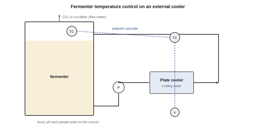
Anaerobic fermentation releases about 500 to 600 kJ per kilogram of glucose fermented, and the code estimates a peak release of about 3 MW in a 2,600 m³ fermenter at its fastest. The fermenter's wall area is far too small to remove that through a jacket, so the plant circulates beer through external plate heat exchangers cooled by cooling-tower water. With a log-mean temperature difference of about 8 K and a heat transfer coefficient around 1.4 kW/m²K, the code gives about 270 m² of plate area per fermenter at peak. In summer the cooling water is warmer and the temperature difference smaller; if the exchangers cannot hold 32 to 34 °C, the yeast suffers, as lesson 5 showed. Plants in warm regions add chillers or larger exchangers for summer, and the heat exchangers must be designed for cleaning, since they are a favourite home for biofilm, as lesson 9 explained.

Instrumentation

Bioreactors are instrumented for temperature, pH, pressure, level, gas flows and, in aerobic vessels, dissolved oxygen and off-gas composition. Temperature is measured with resistance thermometers and controlled by the cooling water flow. pH electrodes must survive cleaning and steam and are calibrated often; pH is controlled by adding acid or base, or, in ethanol mash, set at the cook and allowed to drift. Dissolved oxygen probes, either polarographic or optical, measure the oxygen activity in the broth; they drift and foul and are checked against off-gas balances. Off-gas analysers, measuring oxygen and carbon dioxide, give the oxygen uptake, carbon dioxide evolution and respiratory quotient, which are among the best indicators of what the cells are doing.

The most important variables, cell concentration and substrate and product concentrations, are hard to measure online in a corn mash full of solids. Plants rely on frequent samples analysed in the laboratory, typically by liquid chromatography for sugars, ethanol, glycerol and acids, and on microscope counts for yeast. Some plants use online near-infrared or other spectroscopic analysers calibrated against laboratory data, and soft sensors that estimate unmeasured variables from those that are measured: the carbon dioxide flow from a fermenter, for example, tracks the rate of ethanol production almost exactly, because one is made with the other.

Control strategies

Temperature is controlled by feedback on the exchanger cooling water, often with a cascade from fermenter temperature to beer return temperature to cooling water flow, the kind of cascade Theo designed in CHE-374. In the propagator, dissolved oxygen is controlled by a split-range or sequenced loop that first raises agitator speed, then air flow, then back-pressure as the demand rises, and the sugar feed is adjusted to keep the respiratory quotient near 1, so that the yeast respires rather than ferments. Foam is controlled by a level or conductance probe that triggers antifoam addition, with limits on the total dose because antifoam reduces \(k_La\).

Fermentations are batch processes, so much of their control is sequential: recipes that open and close valves, start agitators, add enzymes and yeast at the right volumes, and run the clean-in-place cycles. These follow the batch control model used in many process industries, with phases, steps and procedures, and the recipe for each fermenter is recorded along with its data so that batches can be compared. When Rosa trials a new yeast, the recipe change goes through management of change, and the batch records are compared with the plant's history to see whether the trial worked.

Monitoring a fermenter bank

Carla's screens show the plant's fermenters side by side: temperature, level, carbon dioxide flow and the last laboratory results for each. She looks first at the carbon dioxide curves. A healthy fermentation rises quickly after fill, peaks at about 15 to 20 hours and declines smoothly; a slow rise means a weak pitch or nutrient shortage; a sharp early drop means a stuck fermentation; a long tail with high lactic acid means contamination. Theo builds a simple tool that overlays each fermenter's curve on the plant's average, so deviations are seen within a few hours instead of at drop. It is the bioprocess equivalent of the alarm management work he did in CHE-374: the goal is to give the operator a few clear signals rather than many numbers.

Pilot plants and their limits

Between Rosa's laboratory fermenters and the plant, many companies keep a pilot plant of a few hundred litres to a few cubic metres, where new processes are run in conditions closer to production. Pilot runs test what the laboratory cannot: mash handling, foam, the behaviour of solids, cleaning, and the response of the culture to realistic mixing times and temperature profiles. Their results still need interpretation, because a pilot vessel mixes faster and cools more easily than a production vessel. Engineers use the pilot plant to find problems early and to measure parameters such as \(k_La\), heat release and yield, and they use correlations and scale-down tests to translate those to production.

Kingfisher Bioenergy has no pilot plant, so Theo's approach to the new propagator is to treat the existing propagator as the pilot: he plans a series of measurements on it, with off-gas analysis, dissolved oxygen, power draw and cell counts, to calibrate the \(k_La\) correlation from lesson 8 at plant scale before the new tank is ordered.

Theo ends the scale-up study with a short checklist he will reuse: choose the criterion that matters for the process; calculate what happens to every other quantity; check mixing time against the fastest biological response; size cooling on the peak with summer water; and confirm the uncertain numbers by measurement on existing plant equipment before buying the new vessel.