Activity coefficient models

Thirteen data points are enough to check the rectifier by hand, but a column simulation needs activity coefficients at every composition and temperature the column visits, thousands of times per run. What it needs is a model: an equation for the excess Gibbs energy as a function of composition, with a few constants fitted to the data. Lesson 6 showed that once \(G^E\) is known, the activity coefficients follow by differentiation, and the Gibbs-Duhem equation is satisfied automatically. This lesson fits the four models most used in practice to Theo's ethanol-water data and compares them.

What a good model must do

A model for \(G^E/RT\) must go to zero at both pure-component ends, because a pure liquid is its own reference. It should fit the data with few parameters, so that the parameters can be determined reliably from limited data. It should extend sensibly from binaries to mixtures of many components, using only binary parameters, because ternary and higher data are rare. And ideally its parameters should change smoothly with temperature, so that a fit at one condition can be used nearby. No model is perfect on all four counts, which is why several remain in use.

Margules and van Laar

The two-parameter Margules equation, dating from 1895, is the simplest useful model: \(G^E/(RTx_1x_2) = A_{21}x_1 + A_{12}x_2\). Its activity coefficients are

The parameters have a direct meaning: \(A_{12} = \ln\gamma_1^\infty\) and \(A_{21} = \ln\gamma_2^\infty\). The van Laar equation, from the early 1910s, writes \(G^E/(RTx_1x_2) = A_{12}A_{21}/(A_{12}x_1 + A_{21}x_2)\), giving

Again \(A_{12}\) and \(A_{21}\) are the logarithms of the infinite-dilution activity coefficients. Both models are flexible enough for many binaries and are easy to fit by hand. Both have a weakness: they have no natural extension to multicomponent mixtures, and their parameters have no built-in temperature dependence.

Local composition models: Wilson, NRTL and UNIQUAC

In 1964 Wilson proposed that the composition of the liquid immediately around a molecule differs from the overall composition, because molecules prefer neighbours with which they interact strongly. Building \(G^E\) on these local compositions gave the Wilson equation, with two binary parameters per pair that represent energy differences between unlike and like interactions, and the pure-component molar volumes. Its form extends naturally to any number of components, and the energy parameters carry a reasonable temperature dependence. Its one serious limitation is that it cannot predict two liquid phases, so it is unsuitable for systems such as ethyl acetate and water.

The non-random two-liquid (NRTL) equation of Renon and Prausnitz (1968) uses the same local-composition idea with an extra non-randomness parameter \(\alpha\), usually fixed between 0.2 and 0.47, and it handles liquid-liquid splitting. The universal quasi-chemical (UNIQUAC) equation of Abrams and Prausnitz (1975) splits \(G^E\) into a combinatorial part, from molecular size and shape, and a residual part, from interaction energies. NRTL and UNIQUAC are the standard property methods in chemical process simulators for polar mixtures at low and moderate pressure.

Fitting the models to ethanol-water

The code fits each model by adjusting its two parameters to minimize the sum of squared errors in \(\ln\gamma_1\) and \(\ln\gamma_2\) over the thirteen points from lesson 6, using a simple Nelder-Mead search. Other objective functions are common, such as errors in vapour composition or in bubble pressure, and they give somewhat different parameters. Ingrid points out that the choice of objective should follow what the model will be used for: for a distillation column, errors in vapour composition matter most.

# Fitting Margules, van Laar, Wilson and NRTL to the ethanol (1) - water (2) activity coefficients
import math
ant = {"e": (8.20417, 1642.89, 230.300), "w": (8.07131, 1730.63, 233.426)}
def psat(c, T):
    A, B, C = ant[c]; return 10 ** (A - B / (T + C)) * 0.133322
P = 101.325
data = [(0.0190, 0.1700, 95.5), (0.0721, 0.3891, 89.0), (0.0966, 0.4375, 86.7), (0.1238, 0.4704, 85.3),
        (0.1661, 0.5089, 84.1), (0.2337, 0.5445, 82.7), (0.3273, 0.5826, 81.5), (0.3965, 0.6122, 80.7),
        (0.5079, 0.6564, 79.8), (0.5732, 0.6841, 79.3), (0.6763, 0.7385, 78.74), (0.7472, 0.7815, 78.41),
        (0.8943, 0.8943, 78.15)]
obs = [(x, math.log(y * P / (x * psat("e", T))), math.log((1 - y) * P / ((1 - x) * psat("w", T))), T) for x, y, T in data]

def margules(p, x, T):
    A12, A21 = p; x2 = 1 - x
    return (x2 ** 2 * (A12 + 2 * (A21 - A12) * x), x * x * (A21 + 2 * (A12 - A21) * x2))
def vanlaar(p, x, T):
    A12, A21 = p; x2 = 1 - x; d = A12 * x + A21 * x2
    return (A12 * (A21 * x2 / d) ** 2, A21 * (A12 * x / d) ** 2)
V1, V2 = 58.68, 18.07
def wilson(p, x, T):
    a12, a21 = p; TK = T + 273.15; x2 = 1 - x
    L12 = V2 / V1 * math.exp(-a12 / (8.314 * TK)); L21 = V1 / V2 * math.exp(-a21 / (8.314 * TK))
    t = L12 / (x + x2 * L12) - L21 / (x2 + x * L21)
    return (-math.log(x + x2 * L12) + x2 * t, -math.log(x2 + x * L21) - x * t)
def nrtl(p, x, T, al=0.3):
    g12, g21 = p; TK = T + 273.15; x2 = 1 - x
    t12, t21 = g12 / (8.314 * TK), g21 / (8.314 * TK)
    G12, G21 = math.exp(-al * t12), math.exp(-al * t21)
    l1 = x2 ** 2 * (t21 * (G21 / (x + x2 * G21)) ** 2 + t12 * G12 / (x2 + x * G12) ** 2)
    l2 = x * x * (t12 * (G12 / (x2 + x * G12)) ** 2 + t21 * G21 / (x + x2 * G21) ** 2)
    return (l1, l2)

def sse(model, p):
    s = 0.0
    for x, l1, l2, T in obs:
        try: m1, m2 = model(p, x, T)
        except (ValueError, ZeroDivisionError, OverflowError): return 1e9
        s += (m1 - l1) ** 2 + (m2 - l2) ** 2
    return s

def nelder_mead(f, p0, step, n=600):
    pts = [list(p0)] + [ [p0[0] + step[0], p0[1]], [p0[0], p0[1] + step[1]]]
    for _ in range(n):
        pts.sort(key=f); best, mid, worst = pts
        c = [(best[i] + mid[i]) / 2 for i in range(2)]
        r = [c[i] + (c[i] - worst[i]) for i in range(2)]
        if f(r) < f(best):
            e = [c[i] + 2 * (c[i] - worst[i]) for i in range(2)]; pts[2] = e if f(e) < f(r) else r
        elif f(r) < f(mid): pts[2] = r
        else:
            k = [c[i] + 0.5 * (worst[i] - c[i]) for i in range(2)]
            if f(k) < f(worst): pts[2] = k
            else: pts = [best] + [ [best[i] + 0.5 * (q[i] - best[i]) for i in range(2)] for q in (mid, worst)]
    pts.sort(key=f); return pts[0]

fits = {}
for name, model, p0, st in (("Margules", margules, (1.5, 0.8), (0.2, 0.2)), ("van Laar", vanlaar, (1.5, 0.9), (0.2, 0.2)),
                            ("Wilson", wilson, (2000, 4000), (500, 500)), ("NRTL", nrtl, (-500, 5000), (500, 500))):
    p = nelder_mead(lambda q: sse(model, q), p0, st)
    fits[name] = (model, p)
    rms = math.sqrt(sse(model, p) / (2 * len(obs)))
    g1inf, g2inf = [math.exp(v) for v in (model(p, 1e-9, 78.3)[0], model(p, 1 - 1e-9, 78.3)[1])]
    print(f"{name:9s} parameters = ({p[0]:.4g}, {p[1]:.4g}), rms ln-gamma error = {rms:.3f}, "
          f"gamma1(inf) = {g1inf:.1f}, gamma2(inf) = {g2inf:.2f}")

# Predicted bubble point and vapour composition at x1 = 0.10 with each model
for name, (model, p) in fits.items():
    lo, hi = 70.0, 100.0
    for _ in range(60):
        T = (lo + hi) / 2; l1, l2 = model(p, 0.10, T)
        f = 0.10 * math.exp(l1) * psat("e", T) + 0.90 * math.exp(l2) * psat("w", T) - P
        lo, hi = (lo, T) if f > 0 else (T, hi)
    y = 0.10 * math.exp(l1) * psat("e", T) / P
    print(f"{name:9s}: x1 = 0.10 boils at {T:.1f} C with y1 = {y:.3f}")

Margules  parameters = (1.6, 0.8134), rms ln-gamma error = 0.022, gamma1(inf) = 5.0, gamma2(inf) = 2.26
van Laar  parameters = (1.672, 0.9304), rms ln-gamma error = 0.015, gamma1(inf) = 5.3, gamma2(inf) = 2.54
Wilson    parameters = (1321, 4011), rms ln-gamma error = 0.018, gamma1(inf) = 6.1, gamma2(inf) = 2.72
NRTL      parameters = (-480.2, 5559), rms ln-gamma error = 0.013, gamma1(inf) = 5.6, gamma2(inf) = 2.49
Margules : x1 = 0.10 boils at 86.6 C with y1 = 0.443
van Laar : x1 = 0.10 boils at 86.6 C with y1 = 0.440
Wilson   : x1 = 0.10 boils at 86.7 C with y1 = 0.434
NRTL     : x1 = 0.10 boils at 86.5 C with y1 = 0.442

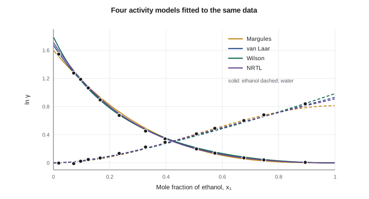
Comparing the fits

All four models fit the data well, with root-mean-square errors in \(\ln\gamma\) of 0.013 to 0.022, about the scatter of the data themselves. NRTL fits best and Margules worst, but the differences are small. Where the models differ is at the edges. Their infinite-dilution activity coefficients of ethanol in water range from 5.0 (Margules) to 6.1 (Wilson), because the data reach only \(x_1 = 0.019\), and each model extrapolates to zero in its own way. Infinite-dilution values matter wherever a component is a trace: in the stripping section of the beer column, where ethanol is removed from water down to about 0.01 %, a 20 % change in \(\gamma_1^\infty\) changes the number of stages needed. When a design depends on the dilute end, Theo notes, the fit should include infinite-dilution data, and Dev can measure \(\gamma^\infty\) directly by gas chromatography.

In the middle of the range the models agree closely. At \(x_1 = 0.10\), all four predict a bubble point of 86.5 to 86.7 °C and a vapour with 43.4 to 44.3 % ethanol, against the measured 86.7 °C and 43.8 % at a nearby composition. For the rectifier, any of them would do. The van Laar fit, with \(A_{12} = 1.672\) and \(A_{21} = 0.930\), is close to the values published for this system decades ago, and lessons 8 and 9 use it because it is simple to write out.

Group contribution: UNIFAC

For a new mixture with no data, such as a bio-based solvent blend the company might sell, the UNIFAC method estimates activity coefficients from the functional groups the molecules contain: CH3, CH2, OH, H2O, CH3COO and so on. It uses UNIQUAC's structure, with group sizes and group-group interaction parameters fitted once to a very large body of data. UNIFAC typically predicts activity coefficients within 10 to 20 % for mixtures similar to those in its database, and much worse for unusual ones. Modified versions, notably the Dortmund version, improve the temperature dependence and the dilute region. UNIFAC is a screening tool: good for comparing options and planning experiments, not for final column design.

Temperature dependence

The parameters fitted here come from isobaric data spanning 78 to 96 °C and are treated as constants. That is reasonable near the fitted range. Further away, the Gibbs-Helmholtz relation of lesson 2 says that \(G^E/RT\) changes with temperature according to the excess enthalpy, and models should then use temperature-dependent parameters, such as \(\tau_{ij} = a_{ij} + b_{ij}/T\) in NRTL. Lesson 10 shows what happens when the 80 °C fit is used at the freezing point.