Modified Raoult's law and activity coefficients

The rectifier at Kingfisher Bioenergy takes a stream of about 40 % ethanol by mass from the beer column and concentrates it to about 95 %. Every tray in it works at the equilibrium between a liquid and a vapour of ethanol and water. Lesson 5 showed that Raoult's law misses that equilibrium badly. Theo pulls the published equilibrium data for ethanol-water at 1 atm from the handbook, and this lesson turns those data into activity coefficients, the correction factors that make Raoult's law work for real liquids.

Activity and the activity coefficient

For a liquid that is not an ideal solution, the fugacity of each component is written as its ideal-solution value times a correction:

The activity coefficient \(\gamma_i\) measures how much more or less the species escapes from the mixture than it would from an ideal solution of the same composition. The product \(a_i = x_i\gamma_i\) is the activity. When \(\gamma_i > 1\), the molecules of \(i\) are less comfortable among their neighbours than among their own kind and escape more readily: a positive deviation from Raoult's law. When \(\gamma_i < 1\), the mixture holds them more tightly: a negative deviation. By definition, \(\gamma_i \to 1\) as \(x_i \to 1\), because a nearly pure liquid is its own ideal solution.

The activity coefficient is connected to the excess Gibbs energy of lesson 2. The partial molar excess Gibbs energy of species \(i\) is \(\bar{G}_i^E = RT\ln\gamma_i\), so the summability relation gives

Activity coefficients therefore obey the Gibbs-Duhem equation: at constant temperature and pressure, \(\sum_i x_i\,d\ln\gamma_i = 0\). For a binary, if \(\gamma_1\) falls as \(x_1\) rises, \(\gamma_2\) must rise in a related way.

Modified Raoult's law

Keeping the ideal-gas vapour and low-pressure liquid fugacity of lesson 5, but using activity coefficients for the liquid, gives the equation used for most low-pressure vapour-liquid equilibrium:

It holds well below a few bar for most chemical systems. At higher pressures the full gamma-phi form adds the vapour fugacity coefficient, \(\phi^{\text{sat}}\) and the Poynting factor: \(y_i\hat{\phi}_iP = x_i\gamma_i\phi_i^{\text{sat}}P_i^{\text{sat}}\exp[V_i^{\text{L}}(P - P_i^{\text{sat}})/RT]\). In this lesson the simple form is enough. The relative volatility now includes the activity coefficients: \(\alpha_{12} = \gamma_1P_1^{\text{sat}}/(\gamma_2P_2^{\text{sat}})\), and because the \(\gamma\) values change with composition, so does \(\alpha\).

Activity coefficients from vapour-liquid data

Rearranging modified Raoult's law gives each activity coefficient directly from one measured point: \(\gamma_i = y_iP/(x_iP_i^{\text{sat}})\), with the vapour pressure evaluated at the measured temperature. This is how activity coefficient data are generated. The code applies it to thirteen published points for ethanol-water at 1 atm, rounded from a standard handbook table.

# Activity coefficients of ethanol (1) and water (2) from isobaric data at 1 atm (modified Raoult's law)
import math
ant = {"ethanol": (8.20417, 1642.89, 230.300), "water": (8.07131, 1730.63, 233.426)}
def psat(c, T):
    A, B, C = ant[c]; return 10 ** (A - B / (T + C)) * 0.133322   # kPa, T in C
P = 101.325
# x1, y1, T/C: published data for ethanol-water at 1 atm, rounded
data = [(0.0190, 0.1700, 95.5), (0.0721, 0.3891, 89.0), (0.0966, 0.4375, 86.7), (0.1238, 0.4704, 85.3),
        (0.1661, 0.5089, 84.1), (0.2337, 0.5445, 82.7), (0.3273, 0.5826, 81.5), (0.3965, 0.6122, 80.7),
        (0.5079, 0.6564, 79.8), (0.5732, 0.6841, 79.3), (0.6763, 0.7385, 78.74), (0.7472, 0.7815, 78.41),
        (0.8943, 0.8943, 78.15)]
print("  x1      T     g1     g2    ln(g1/g2)   GE/RT")
rows = []
for x1, y1, T in data:
    g1 = y1 * P / (x1 * psat("ethanol", T))
    g2 = (1 - y1) * P / ((1 - x1) * psat("water", T))
    ge = x1 * math.log(g1) + (1 - x1) * math.log(g2)
    rows.append((x1, math.log(g1 / g2)))
    print(f"{x1:6.4f}  {T:6.2f}  {g1:5.3f}  {g2:5.3f}  {math.log(g1 / g2):8.3f}  {ge:7.4f}")

# Redlich-Kister area test: the integral of ln(g1/g2) from x1 = 0 to 1 should be close to zero
# (strictly true at constant T; isobaric data pass if the net area is a small fraction of the total)
pts = [(0.0, 2.1)] + rows + [(1.0, -1.0)]       # end values extrapolated by eye from the trend
net = sum((pts[i + 1][0] - pts[i][0]) * (pts[i + 1][1] + pts[i][1]) / 2 for i in range(len(pts) - 1))
tot = sum((pts[i + 1][0] - pts[i][0]) * (abs(pts[i + 1][1]) + abs(pts[i][1])) / 2 for i in range(len(pts) - 1))
print(f"net area = {net:.3f}, total area = {tot:.3f}, ratio = {abs(net) / tot * 100:.0f} %")

# Relative volatility of ethanol to water
for x1, y1, T in (data[1], data[8], data[12]):
    alpha = (y1 / x1) / ((1 - y1) / (1 - x1))
    print(f"x1 = {x1:.4f}: relative volatility = {alpha:.2f}")

  x1      T     g1     g2    ln(g1/g2)   GE/RT
0.0190   95.50  4.688  0.996     1.549   0.0257
0.0721   89.00  3.581  0.990     1.286   0.0824
0.0966   86.70  3.275  1.023     1.164   0.1351
0.1238   85.30  2.897  1.049     1.016   0.1734
0.1661   84.10  2.446  1.071     0.825   0.2060
0.2337   82.70  1.963  1.143     0.541   0.2601
0.3273   81.50  1.571  1.252     0.227   0.2990
0.3965   80.70  1.406  1.339     0.049   0.3112
0.5079   79.80  1.219  1.509    -0.213   0.3030
0.5732   79.30  1.148  1.632    -0.352   0.2883
0.6763   78.74  1.074  1.823    -0.529   0.2426
0.7472   78.41  1.042  1.977    -0.640   0.2031
0.8943   78.15  1.007  2.312    -0.831   0.0946
net area = -0.019, total area = 0.625, ratio = 3 %
x1 = 0.0721: relative volatility = 8.20
x1 = 0.5079: relative volatility = 1.85
x1 = 0.8943: relative volatility = 1.00

What the data show

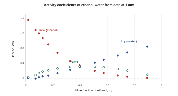
Both activity coefficients are greater than 1 almost everywhere: ethanol-water shows a strong positive deviation. Ethanol is the more non-ideal component, with \(\gamma_1 = 4.7\) at \(x_1 = 0.019\) and an infinite-dilution value of about 5. A few ethanol molecules in a large amount of water escape about five times as readily as Raoult's law expects. Water reaches \(\gamma_2 = 2.3\) near the azeotrope. Two points near the water-rich end show \(\gamma_2\) slightly below 1, which is within the scatter of the data. The excess Gibbs energy \(G^E/RT\) peaks at about 0.31 near \(x_1 = 0.4\), a moderate value. Mixtures with a peak above about 0.5 to 0.7 can split into two liquid phases, as lesson 10 shows for ethyl acetate and water.

The relative volatility of ethanol to water is 8.2 at \(x_1 = 0.072\), which is why the bottom of the rectifier separates easily, 1.85 at \(x_1 = 0.51\), and 1.00 at \(x_1 = 0.894\). A relative volatility of 1 means the vapour and liquid have the same composition: no tray can make further progress, and the column is pinched at the azeotrope. Raoult's law alone, with \(\alpha = P_1^{\text{sat}}/P_2^{\text{sat}}\) between about 2.2 and 2.3 across the range, predicts neither the easy separation at the bottom nor the pinch at the top.

Testing data for thermodynamic consistency

Measured vapour-liquid data contain errors in temperature, pressure and both compositions, and the Gibbs-Duhem equation gives a way to catch them. Integrating \(x_1\,d\ln\gamma_1 + x_2\,d\ln\gamma_2 = 0\) from \(x_1 = 0\) to 1 at constant temperature gives the Redlich-Kister area test:

The plot of \(\ln(\gamma_1/\gamma_2)\) against \(x_1\) should enclose equal areas above and below the axis. For isobaric data, where the temperature changes along the curve, the integral is not exactly zero, and a small residual is accepted. The ethanol-water set gives a net area of about 3 % of the total, which passes the usual screen for isobaric data. The test is necessary rather than sufficient: data can pass it and still contain compensating errors. More detailed point-by-point tests, such as the Van Ness method, compare measured vapour compositions with those predicted from a fitted model, and evaluated databanks apply such tests before a data set is recommended.

Where activity coefficients come from in practice

Activity coefficients are measured, not derived from first principles, and the main sources are vapour-liquid data such as these, infinite-dilution measurements by gas chromatography or ebulliometry, and liquid-liquid solubility data. Large evaluated collections, such as the DECHEMA Chemistry Data Series and the Dortmund Data Bank, hold many thousands of binary data sets. When a system has never been measured, group-contribution methods such as UNIFAC estimate activity coefficients from the chemical groups in the molecules, which lesson 7 describes. Dev's lab can measure a few points for an unusual mixture in a day with a small recirculating still, and Theo notes that this is cheaper than a column that does not work.

Activity on other scales

The activity coefficient in this lesson uses the pure liquid at the system temperature as its standard state, the convention natural for components that are liquids. For dissolved gases and for solids dissolved in liquids, other conventions are used: the Henry's law standard state, in which \(\gamma_i^* \to 1\) as \(x_i \to 0\), and molality-based scales for electrolytes. Each convention gives a different numerical activity coefficient for the same physical state, but consistent calculations give the same equilibrium. Lesson 10 uses the pure-component convention for liquid-liquid equilibrium.

Activity coefficients and the column

The practical value of activity coefficients shows up in the number of stages a column needs. Theo runs a quick comparison. Separating a 10 mol % ethanol feed into 80 mol % overhead and almost pure water at the bottom needs, with Raoult's law and a constant relative volatility of about 2.3, about ten theoretical stages at total reflux by the Fenske equation. With the measured activity coefficients, the bottom section separates much more easily, because the relative volatility there is about 8, and the top section much less easily, because it falls toward 1 as the composition approaches the azeotrope. The real column has a few stages doing most of the work at the bottom and many stages crawling toward 80 % near the top. A design based on Raoult's law would get the stage count wrong in both sections and would never reveal the azeotrope barrier. CHE-350 builds stage-by-stage designs on exactly these data.

Negative deviations and what they mean

Not every mixture shows positive deviations. When unlike molecules attract each other more strongly than like ones, activity coefficients fall below 1 and partial pressures fall below Raoult's law. Acetone with chloroform is the textbook case: the hydrogen on chloroform bonds to the oxygen of acetone, and the mixture boils above both pure components at some compositions. Water with strong acids such as nitric or hydrochloric acid behaves the same way. In the ethyl acetate line, acetic acid with water shows only small deviations, while acetic acid in the vapour forms dimers, a different kind of non-ideality that lesson 12 mentions. Knowing the sign of the deviation tells the engineer what kind of azeotrope, if any, to expect.

A useful way to picture the sign is through the excess Gibbs energy. Positive \(G^E\) means the mixture is less stable than an ideal solution: the molecules would rather be with their own kind, and if \(G^E\) is large enough they separate into two liquids, as lesson 10 shows. Negative \(G^E\) means the mixture is more stable than ideal and never splits. Ethanol-water, with \(G^E/RT\) peaking at 0.31, sits comfortably in the miscible range despite its strong positive deviations.