Fugacity in mixtures and mixing rules

The gas leaving the Lakeshore Gas first-stage cooler is not pure carbon dioxide. After the CHE-314 scrubber and compression to 20 bar at 35 °C it still carries traces of ethanol and water, roughly 0.4 and 0.2 mol %. Those traces decide whether liquid drops out in the next cooler and how big the dryer must be. To answer, Theo needs the fugacity of each component in the mixture, not just the fugacity of pure carbon dioxide. This lesson extends lesson 3 from pure fluids to mixtures.

Fugacity of a species in a mixture

For a species \(i\) in a mixture, the fugacity \(\hat{f}_i\) is defined in the same way as for a pure fluid, with the chemical potential of that species: \(d\mu_i = RT\,d\ln\hat{f}_i\) at constant temperature. For an ideal-gas mixture, \(\hat{f}_i = y_iP\), the partial pressure. For a real gas mixture, the fugacity coefficient of the species in solution is

The hat is a reminder that this is a property of a species in a mixture, not of the pure substance. The condition of phase equilibrium in its working form is equality of \(\hat{f}_i\) in every phase. For vapour-liquid equilibrium, that is

There are two ways to evaluate the liquid side. The gamma-phi approach writes the liquid fugacity with an activity coefficient, \(\hat{f}_i^{\,\text{L}} = x_i\gamma_i f_i\), and the vapour with a fugacity coefficient; lessons 5 to 8 use it at low pressure. The phi-phi approach uses one equation of state for both phases, \(y_i\hat{\phi}_i^{\,\text{V}} = x_i\hat{\phi}_i^{\,\text{L}}\); lesson 9 uses it at high pressure. Both need a way to apply an equation of state to a mixture.

The ideal solution and the Lewis-Randall rule

The simplest mixture model assumes that every component's fugacity is proportional to its mole fraction, with the pure-component fugacity at the same temperature and pressure as the constant: \(\hat{f}_i^{\,\text{id}} = y_i f_i\). This is the Lewis-Randall rule, and it defines the ideal solution. For gases it means \(\hat{\phi}_i = \phi_i\): each component has the fugacity coefficient it would have if pure at the mixture's \(T\) and \(P\). The rule is exact for an ideal-gas mixture and reasonable for mixtures of similar molecules, such as nitrogen and oxygen, or methane and ethane at modest pressure. It fails in two ways that matter in the plant. It cannot handle components whose pure form at \(T\) and \(P\) would be a liquid, such as ethanol and water in compressed carbon dioxide, because there is no pure gas fugacity to use. And it ignores the unlike interactions between different molecules, which are exactly what make mixtures interesting.

Mixing rules for cubic equations

A cubic equation of state is extended to mixtures by giving the mixture its own constants \(a\) and \(b\), built from the pure-component values by mixing rules. The van der Waals one-fluid rules are the standard:

The geometric mean for \(a_{ij}\) reflects the idea that the attraction between unlike molecules is roughly the geometric mean of the like attractions; the binary interaction parameter \(k_{ij}\) corrects it. Typical \(k_{ij}\) values are zero for hydrocarbon pairs of similar size, about 0.1 to 0.15 for carbon dioxide with hydrocarbons, and larger and temperature-dependent for water with almost anything. They are fitted to binary data, and process simulators carry tables of them. With \(a_m\) and \(b_m\), the cubic gives the mixture compressibility \(Z\), and differentiation gives each component's fugacity coefficient:

The structure of this expression is worth noticing. The term \(\sum_j y_ja_{ij}\) is the average attraction felt by a molecule of \(i\) from its neighbours. In a gas that is mostly carbon dioxide, an ethanol molecule's neighbours are carbon dioxide molecules, and the result depends on the ethanol-carbon dioxide interaction, not on the ethanol-ethanol attraction that the Lewis-Randall rule would use.

# Fugacity coefficients in a gas mixture with the Peng-Robinson equation and van der Waals mixing rules
import math
R = 8.314  # J/(mol K)

def pr_params(Tc, Pc, w, T):
    kappa = 0.37464 + 1.54226 * w - 0.26992 * w * w
    alpha = (1 + kappa * (1 - math.sqrt(T / Tc))) ** 2
    a = 0.45724 * R * R * Tc * Tc / Pc * alpha
    b = 0.07780 * R * Tc / Pc
    return a, b

def cubic_roots(c2, c1, c0):
    # real roots of Z^3 + c2 Z^2 + c1 Z + c0 = 0 (Cardano with trigonometric form)
    q = (3 * c1 - c2 * c2) / 9; r = (9 * c2 * c1 - 27 * c0 - 2 * c2 ** 3) / 54
    d = q ** 3 + r * r
    if d > 0:
        s = math.copysign(abs(r + math.sqrt(d)) ** (1 / 3), r + math.sqrt(d))
        t = math.copysign(abs(r - math.sqrt(d)) ** (1 / 3), r - math.sqrt(d))
        return [s + t - c2 / 3]
    th = math.acos(r / math.sqrt(-q ** 3))
    return sorted(2 * math.sqrt(-q) * math.cos((th + 2 * math.pi * k) / 3) - c2 / 3 for k in range(3))

def pr_Z(A, B):
    return cubic_roots(-(1 - B), A - 3 * B * B - 2 * B, -(A * B - B * B - B ** 3))

def pr_lnphi_pure(Z, A, B):
    s2 = math.sqrt(2)
    return Z - 1 - math.log(Z - B) - A / (2 * s2 * B) * math.log((Z + (1 + s2) * B) / (Z + (1 - s2) * B))
comps = ["CO2", "ethanol", "water"]
Tc = [304.13, 513.9, 647.1]; Pc = [73.77e5, 61.48e5, 220.64e5]; w = [0.225, 0.645, 0.345]
kij = [ [0, 0.09, 0.12], [0.09, 0, -0.08], [0.12, -0.08, 0]]   # illustrative binary parameters
y = [0.994, 0.004, 0.002]
T, P = 308.15, 20e5                                            # 35 C, 20 bar

ab = [pr_params(Tc[i], Pc[i], w[i], T) for i in range(3)]
a = [p[0] for p in ab]; b = [p[1] for p in ab]

def mix_phi(y, kij):
    aij = [ [math.sqrt(a[i] * a[j]) * (1 - kij[i][j]) for j in range(3)] for i in range(3)]
    am = sum(y[i] * y[j] * aij[i][j] for i in range(3) for j in range(3))
    bm = sum(y[i] * b[i] for i in range(3))
    A = am * P / (R * T) ** 2; B = bm * P / (R * T)
    Z = max(pr_Z(A, B)); s2 = math.sqrt(2)
    out = []
    for i in range(3):
        sa = sum(y[j] * aij[i][j] for j in range(3))
        lnphi = (b[i] / bm * (Z - 1) - math.log(Z - B)
                 - A / (2 * s2 * B) * (2 * sa / am - b[i] / bm) * math.log((Z + (1 + s2) * B) / (Z + (1 - s2) * B)))
        out.append(math.exp(lnphi))
    return Z, out

Z, phis = mix_phi(y, kij)
print(f"mixture Z = {Z:.4f}")
for c, yi, ph in zip(comps, y, phis):
    print(f"{c:8s} y = {yi:.3f}  phi = {ph:.4f}  fugacity = {yi * ph * 20:.4f} bar")

Z0, phis0 = mix_phi(y, [ [0] * 3 for _ in range(3)])
print("with all kij = 0: " + ", ".join(f"{c} {p:.4f}" for c, p in zip(comps, phis0)))

# Lewis-Randall rule: phi_i(mixture) = phi of pure i at the same T and P
a0, b0 = ab[0]
A = a0 * P / (R * T) ** 2; B = b0 * P / (R * T)
print(f"Lewis-Randall for CO2: phi = {math.exp(pr_lnphi_pure(max(pr_Z(A, B)), A, B)):.4f}")
for i in (1, 2):
    A = a[i] * P / (R * T) ** 2; B = b[i] * P / (R * T)
    roots = pr_Z(A, B)
    print(f"pure {comps[i]} at 35 C and 20 bar has {len(roots)} real root(s), smallest Z = {min(roots):.4f}: it is a liquid, so the rule has no gas value to use")

mixture Z = 0.8947
CO2      y = 0.994  phi = 0.9038  fugacity = 17.9667 bar
ethanol  y = 0.004  phi = 0.6815  fugacity = 0.0545 bar
water    y = 0.002  phi = 0.8099  fugacity = 0.0324 bar
with all kij = 0: CO2 0.9038, ethanol 0.6448, water 0.7716
Lewis-Randall for CO2: phi = 0.9037
pure ethanol at 35 C and 20 bar has 1 real root(s), smallest Z = 0.0492: it is a liquid, so the rule has no gas value to use
pure water at 35 C and 20 bar has 1 real root(s), smallest Z = 0.0167: it is a liquid, so the rule has no gas value to use

What the results show

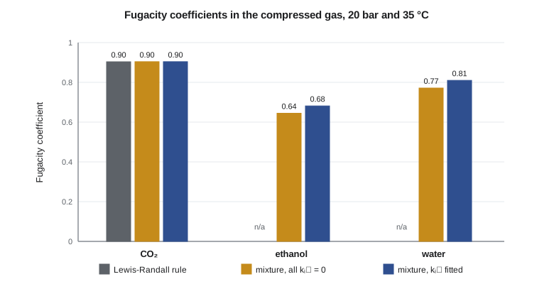
The mixture is 99.4 % carbon dioxide, so its compressibility, 0.895, is almost that of the pure gas, and the carbon dioxide fugacity coefficient, 0.904, is the same as in lesson 3. Here the Lewis-Randall rule would have been fine. The trace components are different. Ethanol has \(\hat{\phi} = 0.68\) and water 0.81, well below the carrier's value, because these polar molecules are strongly attracted by their neighbours, which lowers their escaping tendency. Their fugacities, 0.055 bar for ethanol and 0.032 bar for water, are the quantities to compare with the fugacity of liquid ethanol or water at 35 °C to decide whether either will condense.

The interaction parameters used in the code are illustrative values of the right size, not fitted constants, and the results show how much they matter. Setting all \(k_{ij}\) to zero changes the ethanol coefficient from 0.68 to 0.64 and the water coefficient from 0.81 to 0.77, changes of about 5 %, which translate directly into a 5 % error in the predicted dew point composition. For a dryer sized on water content, 5 % is tolerable; for a high-purity product specification it may not be. Theo notes in his calculations that the \(k_{ij}\) values must come from the simulator's fitted database before the numbers are used for design.

Other mixing rules

The one-fluid van der Waals rules work well for nonpolar and mildly polar mixtures. For mixtures of a gas with strongly polar liquids, such as carbon dioxide with water and alcohols, more flexible rules are used. The Wong-Sandler and MHV2 rules build the mixture \(a\) parameter from an excess Gibbs energy model of the kind lesson 7 introduces, so that the equation of state reproduces liquid activity coefficients at low pressure while keeping its proper behaviour at high pressure. Predictive versions such as PSRK combine the Soave equation with the UNIFAC group contribution method. Simulators offer these as separate property methods, and choosing among them is part of lesson 12.

The residual Gibbs energy view

Another way to see the fugacity coefficient is as a residual property. The residual Gibbs energy of a fluid is the difference between its Gibbs energy and that of an ideal gas at the same temperature, pressure and composition: \(G^R = G - G^{\text{ig}}\). For a pure fluid, \(G^R/RT = \ln\phi\); for a mixture, \(\ln\hat{\phi}_i\) is the partial molar residual Gibbs energy divided by \(RT\). The same equation of state that gives \(\phi\) also gives the residual enthalpy and entropy used in Thermodynamics I for compression work. One consistent model supplies phase equilibrium and energy balances, which is why simulators are built around property packages rather than separate correlations.