Convective mass transfer and mass transfer coefficients

The yeast propagation tanks at Kingfisher Bioenergy are small compared with the fermenters, but they matter: they grow the yeast population that seeds every fermentation batch, and yeast grow well only with oxygen. During a hot spell last summer the propagation batches came out weak, and the plant manager asked process engineering whether the tanks get enough oxygen. Ingrid gives the question to Theo, along with data from a test the operators ran with the dissolved oxygen probe. Answering it needs the idea at the heart of practical mass transfer: the mass transfer coefficient, and the models that explain what it depends on.

Why coefficients

Molecular diffusion in a moving fluid is described exactly by the convection-diffusion equation, but solving it requires the full velocity field, which is rarely known in turbulent flow or in a stirred tank with bubbles. Engineers sidestep the problem the same way heat transfer does. They define a coefficient that relates the flux at an interface to a simple driving force between the interface and the bulk fluid, and then measure or correlate that coefficient. For the liquid side of a gas-liquid interface,

where \(c_{Ai}\) is the concentration at the interface and \(c_{AL}\) is the bulk liquid concentration. The coefficient \(k_L\) has units of m/s, like a velocity. On the gas side, the coefficient is defined with whatever driving force is convenient. The relations between the most common forms come straight from \(c_A = p_A/RT = y_A c\):

In the liquid phase, \(k_x = c_L k_L\) for a mole fraction driving force, where \(c_L\) is the total molar concentration of the liquid, about 55,000 mol/m\(^3\) for water. Mixing up these forms is one of the commonest errors in mass transfer calculations, because the numbers differ by large factors. A gas-side coefficient of 0.02 m/s at 32 °C is the same as \(k_y = 0.80\) mol/(m\(^2\) s) and \(k_G = 7.9\times10^{-6}\) mol/(m\(^2\) s Pa).

For concentrated systems where only one species crosses the interface, the bulk-flow effect from lesson 3 is often absorbed into the coefficient. Textbooks then distinguish \(k'_y\), for equimolar counterdiffusion, from \(k_y = k'_y/y_{B,\mathrm{lm}}\), for diffusion through a stagnant component. For dilute solutes, as in the scrubber and the propagation tank, the difference is small and this course does not track it separately.

Film theory

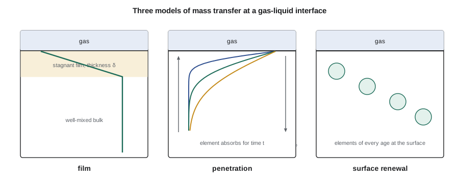
The simplest model, proposed by Whitman in the 1920s, imagines that all the resistance to mass transfer lies in a thin stagnant film of thickness \(\delta\) next to the interface, with the fluid beyond it perfectly mixed. Diffusion across the film is steady, so from lesson 3,

The film thickness is not a real, measurable layer; it is the thickness a stagnant film would need to have to give the observed coefficient. Film theory predicts that \(k\) is proportional to \(D_{AB}\). Experiments on liquids usually show a weaker dependence, closer to \(D_{AB}^{1/2}\) to \(D_{AB}^{2/3}\), which is the first hint that the picture is too simple. Its great value is that it is easy to use and gives the right structure for combining resistances in series, which lesson 7 relies on.

Penetration and surface renewal theories

In 1935 Higbie argued that at many gas-liquid interfaces, such as the surface of a rising bubble or liquid flowing over packing, the liquid near the surface is never at steady state. Each small element of liquid arrives at the interface, absorbs gas for a short contact time \(t_e\) as if it were a semi-infinite medium, and is then swept away into the bulk. Using the erfc solution from lesson 4 and averaging the flux over the contact time gives

Danckwerts refined the idea in 1951. Instead of a fixed contact time, surface elements are replaced at random, with a fractional rate of surface renewal \(s\), so elements of every age are present at the surface. Averaging over that age distribution gives \(k_L = \sqrt{D_{AB}\,s}\). Both theories predict \(k_L \propto D_{AB}^{1/2}\), close to many measurements in agitated liquids and packed columns. Neither the contact time nor the renewal rate can be predicted from first principles for most equipment, so the theories are used mainly to understand trends and to extrapolate measured coefficients from one solute to another. If oxygen's \(k_L\) has been measured, the value for carbon dioxide in the same equipment is about \(k_{L,\mathrm{O_2}}\sqrt{D_{\mathrm{CO_2}}/D_{\mathrm{O_2}}}\).

Volumetric coefficients and kLa

In bubble columns, stirred tanks and packed beds, the interfacial area is hard to measure separately from the coefficient. The two are therefore combined into a volumetric coefficient: \(k_La\) for the liquid side, where \(a\) is the interfacial area per unit volume of liquid or of equipment, in m\(^2\)/m\(^3\). The transfer rate per unit volume is then

for oxygen, where \(C^*\) is the dissolved oxygen concentration in equilibrium with the gas and \(C_L\) is the actual concentration in the broth. Oxygen is only sparingly soluble, about 7 to 8 mg/L in water in equilibrium with air near room temperature and less in warm broth, so the driving force is small and \(k_La\) must be large. Gas-side resistance is negligible for oxygen because it is so poorly soluble, a point lesson 7 makes precise. Typical \(k_La\) values range from a few per hour in gently aerated tanks to several hundred per hour in vigorously agitated fermenters.

At steady state the oxygen transfer rate must equal the oxygen uptake rate (OUR) of the yeast. Rearranging gives the \(k_La\) a tank must deliver to hold a chosen dissolved oxygen level: \(k_La = \text{OUR}/(C^* - C_L)\). Raising the temperature hurts twice: oxygen solubility falls, shrinking the driving force, and the yeast grow faster and need more oxygen.

Measuring kLa: the dynamic method

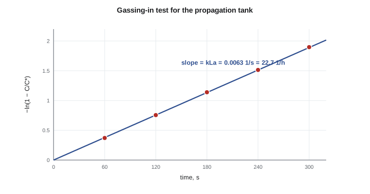
The operators' test used the dynamic gassing-in method. They stripped the oxygen from a batch of medium with nitrogen, then switched to air at the normal flow and agitation and logged the dissolved oxygen as it rose. With no consumption, the balance is \(dC_L/dt = k_La(C^* - C_L)\), whose solution is \(\ln[C^*/(C^* - C_L)] = k_La\,t\). A plot of \(-\ln(1 - C_L/C^*)\) against time is a straight line through the origin whose slope is \(k_La\). In practice the probe has its own response time, a few seconds to tens of seconds, and the first points are often discarded or corrected for it.

# Mass transfer coefficients: unit conversions, film and penetration models,
# and oxygen transfer in the yeast propagation tank
import math
R, T, P = 8.314, 305.15, 101325.0
c = P / (R * T)
kc = 0.020                      # m/s, gas-phase coefficient with concentration driving force
ky = kc * c                     # mol/(m2 s) per unit mole fraction
kG = kc / (R * T)               # mol/(m2 s Pa)
print(f"k_c = {kc} m/s -> k_y = {ky:.3f} mol/(m2 s) -> k_G = {kG:.2e} mol/(m2 s Pa)")

# Film theory versus penetration theory for oxygen absorbing into water
D = 2.4e-9                      # m2/s, oxygen in water at 32 C (approximate)
delta = 20e-6                   # m, film thickness
kL_film = D / delta
t_e = 0.10                      # s, contact time of a surface element
kL_pen = 2 * math.sqrt(D / (math.pi * t_e))
s = 10.0                        # 1/s, surface renewal rate
kL_sr = math.sqrt(D * s)
print(f"film kL = {kL_film:.2e}, penetration kL = {kL_pen:.2e}, surface renewal kL = {kL_sr:.2e} m/s")
D2 = 1.9e-9                     # m2/s, a solute with lower diffusivity
print(f"ratio kL(O2)/kL(other): film {D / D2:.2f}, penetration {math.sqrt(D / D2):.2f}")

# Oxygen transfer rate in the propagation tank
C_sat = 7.3e-3                  # kg/m3, O2 solubility in the mash with air (approximate)
C_L = 1.5e-3                    # kg/m3, dissolved O2 held by control
OUR = 0.10                      # kg O2/(m3 h), oxygen demand of the growing yeast
kLa_needed = OUR / (C_sat - C_L)
print(f"required kLa = {kLa_needed:.1f} 1/h = {kLa_needed / 3600:.4f} 1/s")
V = 200.0                       # m3 working volume
print(f"oxygen to transfer = {OUR * V:.1f} kg/h")

# Dynamic gassing-in test: estimate kLa from DO readings (fraction of saturation vs time)
times = [0, 60, 120, 180, 240, 300]          # s
frac = [0.00, 0.31, 0.53, 0.68, 0.78, 0.85]  # C/C* readings
num = den = 0.0
for t, f in zip(times[1:], frac[1:]):
    yv = -math.log(1 - f)
    num += t * yv; den += t * t
kla = num / den
print(f"kLa from the gassing-in test = {kla:.4f} 1/s = {kla * 3600:.1f} 1/h")

k_c = 0.02 m/s -> k_y = 0.799 mol/(m2 s) -> k_G = 7.88e-06 mol/(m2 s Pa)
film kL = 1.20e-04, penetration kL = 1.75e-04, surface renewal kL = 1.55e-04 m/s
ratio kL(O2)/kL(other): film 1.26, penetration 1.12
required kLa = 17.2 1/h = 0.0048 1/s
oxygen to transfer = 20.0 kg/h
kLa from the gassing-in test = 0.0063 1/s = 22.7 1/h

The results answer the plant manager's question. To hold the dissolved oxygen at 1.5 mg/L with an uptake of 0.10 kg O\(_2\)/(m\(^3\) h), the tank needs \(k_La\) of about 17 h\(^{-1}\). The gassing-in test gives about 23 h\(^{-1}\), a margin of roughly 30 % at the test temperature. On the hottest days, though, the broth was warmer, the oxygen solubility lower and the yeast hungrier, and that margin disappears. Theo recommends raising the air flow during hot weather and checking the sparger, which had partly plugged holes at the last inspection.

There is one more subtlety in the test. The dissolved oxygen probe itself has a membrane through which oxygen must diffuse, so it responds with a time constant of its own, typically several seconds. If that time constant is not small compared with \(1/k_La\), the measured rise is slowed and \(k_La\) is underestimated. For the propagation tank, \(1/k_La\) is about 160 seconds, much longer than the probe's response, so the correction is small. In large, well-mixed fermenters with \(k_La\) above 300 h\(^{-1}\), \(1/k_La\) falls to around 10 seconds and the probe response must be included in the fit.

Using coefficients well

Mass transfer coefficients carry their history with them: the flow, the geometry and the fluid properties at which they were measured. They transfer reliably to new conditions only through correlations in dimensionless groups, which lesson 6 develops, or through models such as penetration theory that say how they should scale. A coefficient quoted without its driving-force definition, units and conditions is not a number a designer can use. Theo's notes for this lesson end with a short checklist: what driving force, what units, what interfacial area basis, what temperature, and measured or correlated.