Internal forced convection

Inside every pipe and tube at Northgate, a fluid flows and exchanges heat with the wall: district water in the transmission main, steam in the converters, glycol in the chilled-water loops, and oil in the heat-transfer systems of two industrial customers on the network. Internal flow differs from external flow in one essential way. The boundary layers grow from the walls until they meet at the centre of the tube, after which the flow is fully developed and confined. The fluid's mean temperature then changes along the tube as it gains or loses heat, so the temperature difference driving convection is not constant. This lesson develops the tools for internal flow: the mean temperature, entry lengths, the energy balance along a tube and the correlations for laminar and turbulent flow.

Hydrodynamic and thermal entry

Fluid entering a tube with a uniform velocity develops a boundary layer on the wall. In laminar flow the boundary layer fills the tube after a hydrodynamic entry length of about \(0.05\,\text{Re}_D D\), and the velocity profile becomes parabolic. Similarly, a thermal boundary layer grows from a heated or cooled wall and fills the tube after a thermal entry length of about \(0.05\,\text{Re}_D\text{Pr}\,D\). For gases these lengths are similar; for oils, with Prandtl numbers in the hundreds, the thermal entry length can be enormous, so the whole tube may lie in the developing region. In turbulent flow both entry lengths are short, roughly 10 to 60 diameters, and fully developed conditions are usually assumed.

The Reynolds number for a circular tube is \(\text{Re}_D = \rho u_m D/\mu = 4\dot m/(\pi D\mu)\), based on the mean velocity. Flow is laminar below about 2300 and fully turbulent above about 10,000, with a transitional range between in which predictions are uncertain. For non-circular ducts, the hydraulic diameter \(D_h = 4A_c/P\) is used in place of \(D\), which works well for turbulent flow and less well for laminar flow in sharp-cornered ducts.

Mean temperature and the energy balance

Because the temperature varies across the tube, a single representative value is needed. The mean (or bulk) temperature \(T_m\) is defined so that \(\dot m c_p T_m\) equals the rate at which the flow carries thermal energy; physically it is the temperature you would measure if you collected the fluid at that section in a cup and mixed it. An energy balance on the whole tube links the heat transferred to the change in mean temperature:

and an energy balance on a slice of length \(dx\) gives \(\dot m c_p\,dT_m = q_s''\,P\,dx\), where \(P\) is the perimeter. Two boundary conditions dominate practice. With a uniform surface heat flux, as from electric heating or a uniformly heated nuclear fuel pin, \(T_m\) rises linearly along the tube. With a uniform surface temperature, as in a tube surrounded by condensing steam or boiling liquid, the difference \(T_s - T_m\) decays exponentially:

The log-mean temperature difference \(\Delta T_{\text{lm}}\) is the correct average driving force for a tube with a uniform wall temperature, and it reappears in heat exchanger analysis in Lesson 12. Using the arithmetic mean instead overestimates the heat rate when the inlet and outlet differences are very different. When the outside of the tube is not isothermal but exchanges heat with a surrounding fluid through insulation, as with a buried pipe, the same exponential applies with \(\bar h P\) replaced by the overall conductance per unit length, \(UP\) or \(1/R'\), and \(T_s\) replaced by the outside temperature.

Laminar flow

For fully developed laminar flow in a circular tube, the Nusselt number is a constant: \(\text{Nu}_D = 4.36\) for uniform surface heat flux and \(\text{Nu}_D = 3.66\) for uniform surface temperature. These exact results mean that \(h = \text{Nu}\,k/D\) is independent of velocity, and that small tubes give high coefficients. In the entry region the coefficient is higher, because the thermal boundary layer is thin. For a thermally developing flow with a uniform wall temperature, the Hausen correlation gives the average Nusselt number in terms of the Graetz number \(\text{Gz}_D = (D/L)\,\text{Re}_D\text{Pr}\):

For non-circular ducts, fully developed laminar Nusselt numbers are tabulated by shape; for a square duct with uniform wall temperature it is about 2.98, and for parallel plates with both walls at the same uniform temperature it is 7.54, based on the hydraulic diameter, which is twice the plate spacing.

Turbulent flow

For fully developed turbulent flow in smooth tubes, the classic Dittus-Boelter equation is

valid for \(\text{Re}_D > 10{,}000\), \(0.6 < \text{Pr} < 160\) and moderate temperature differences. Its errors can reach 25 percent. The Gnielinski correlation is more accurate, typically within 10 percent, and covers the transitional range from about 3000:

where \(f\) is the Darcy friction factor, here from Petukhov's formula for smooth tubes; for rough tubes, the friction factor from the Colebrook equation or the Moody chart can be used, which accounts approximately for roughness raising heat transfer along with friction. The friction factor also gives the pressure drop, \(\Delta p = f\,(L/D)\,\rho u_m^2/2\), which sets the pumping power. The close link between friction and heat transfer is no accident: the same turbulent eddies carry momentum and heat, an idea known as the Reynolds analogy.

# Internal forced convection: district water in a transmission main and oil heated by steam in a tube
import math
# Saturated liquid water (approximate table values): T (C), rho, cp, k, mu
WATER = [(20, 998.0, 4182, 0.598, 1.002e-3), (40, 992.0, 4179, 0.631, 0.653e-3), (60, 983.0, 4185, 0.654, 0.467e-3),
         (80, 972.0, 4197, 0.670, 0.355e-3), (100, 958.0, 4217, 0.679, 0.282e-3), (120, 943.0, 4244, 0.683, 0.232e-3)]
def water(T):
    for a, b in zip(WATER, WATER[1:]):
        if a[0] <= T <= b[0]:
            f = (T - a[0]) / (b[0] - a[0])
            return tuple(x + f * (y - x) for x, y in zip(a[1:], b[1:]))
    raise ValueError("temperature outside table")

def gnielinski(Re, Pr):
    f = (0.790 * math.log(Re) - 1.64) ** -2               # Petukhov friction factor, smooth tube
    return f, (f / 8) * (Re - 1000) * Pr / (1 + 12.7 * (f / 8) ** 0.5 * (Pr ** (2/3) - 1))

# 1. The 110 C supply main, DN200, at winter and summer flows
D, L = 0.2073, 1800.0
rho, cp, k, mu = water(110.0); Pr = mu * cp / k
UA_per_m = 49.4 / (110 - (-5))                           # buried-pipe value from Lesson 4, W/m.K
for V in (1.5, 0.2):
    m = rho * V * math.pi / 4 * D**2
    Re = rho * V * D / mu
    f, Nu_g = gnielinski(Re, Pr)
    Nu_db = 0.023 * Re**0.8 * Pr**0.4
    dp = f * L / D * rho * V**2 / 2
    T_out = -5 + (110 - (-5)) * math.exp(-UA_per_m * L / (m * cp))
    print(f"V = {V:.1f} m/s: m = {m:5.1f} kg/s, Re = {Re:.2e}, Nu Gnielinski {Nu_g:6.0f}, Dittus-Boelter {Nu_db:6.0f}, "
          f"h = {Nu_g*k/D:5.0f} W/m2.K")
    print(f"             friction f = {f:.4f}, pressure drop over {L/1000:.1f} km = {dp/1000:6.1f} kPa, "
          f"water arrives at {T_out:.2f} C")

# 2. Laminar heat-transfer oil heated by condensing steam in a 25 mm tube (constant surface temperature)
rho_o, cp_o, k_o, mu_o = 860.0, 2000.0, 0.13, 0.020    # approximate oil properties at the mean temperature
Do, mdot, Ts, Ti = 0.025, 0.10, 150.0, 40.0
Re_o = 4 * mdot / (math.pi * Do * mu_o); Pr_o = mu_o * cp_o / k_o
print(f"\noil: Re = {Re_o:.0f} (laminar), Pr = {Pr_o:.0f}, thermal entry length about {0.05*Re_o*Pr_o*Do:.0f} m")
for Lt in (3.0, 6.0, 12.0):
    Gz = Do / Lt * Re_o * Pr_o
    Nu = 3.66 + 0.0668 * Gz / (1 + 0.04 * Gz**(2/3))     # Hausen, combined entry (thermally developing)
    h = Nu * k_o / Do
    To = Ts - (Ts - Ti) * math.exp(-math.pi * Do * Lt * h / (mdot * cp_o))
    q = mdot * cp_o * (To - Ti)
    print(f"  tube {Lt:4.1f} m: Gz = {Gz:6.0f}, Nu = {Nu:5.2f}, h = {h:5.1f} W/m2.K, outlet {To:5.1f} C, duty {q/1000:4.1f} kW "
          f"(fully developed Nu = 3.66 would give {Ts-(Ts-Ti)*math.exp(-math.pi*Do*Lt*3.66*k_o/Do/(mdot*cp_o)):5.1f} C)")

V = 1.5 m/s: m =  48.1 kg/s, Re = 1.15e+06, Nu Gnielinski   2216, Dittus-Boelter   1957, h =  7279 W/m2.K
             friction f = 0.0114, pressure drop over 1.8 km =  105.4 kPa, water arrives at 109.56 C
V = 0.2 m/s: m =   6.4 kg/s, Re = 1.53e+05, Nu Gnielinski    413, Dittus-Boelter    390, h =  1358 W/m2.K
             friction f = 0.0165, pressure drop over 1.8 km =    2.7 kPa, water arrives at 106.77 C

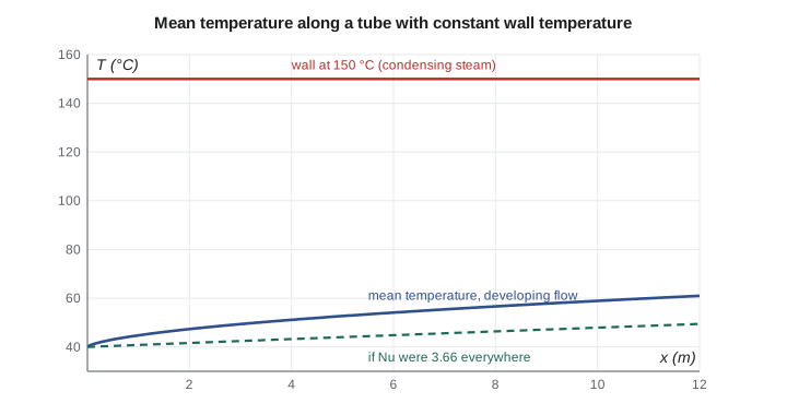
oil: Re = 255 (laminar), Pr = 308, thermal entry length about 98 m
  tube  3.0 m: Gz =    653, Nu = 14.54, h =  75.6 W/m2.K, outlet  49.4 C, duty  1.9 kW (fully developed Nu = 3.66 would give  42.4 C)
  tube  6.0 m: Gz =    326, Nu = 11.19, h =  58.2 W/m2.K, outlet  54.1 C, duty  2.8 kW (fully developed Nu = 3.66 would give  44.8 C)
  tube 12.0 m: Gz =    163, Nu =  8.63, h =  44.9 W/m2.K, outlet  61.0 C, duty  4.2 kW (fully developed Nu = 3.66 would give  49.4 C)

At summer flow, when the network carries only domestic hot water loads, the velocity in the same main may fall to 0.2 m/s. The program shows the consequences: the Reynolds number drops to about 150,000, still turbulent; the pressure drop falls almost fifty-fold; and the water arriving at the hospital is now about 3 K cooler than it left the plant, because the same heat loss is spread over one-seventh of the flow. This is why district systems lose a larger fraction of their heat in summer, and why some utilities lower supply temperatures or use bypasses during low-load periods.

For chemical and process engineers in Canada, the same correlations underlie the heat exchanger design software used across the oil sands, refining and petrochemical industries in Alberta and elsewhere, where heavy, viscous streams often flow in the laminar or transitional range. Pressure vessels and piping for these services are designed and registered under provincial safety authorities using the CSA B51 code and the ASME codes it references.