
CHE-200 · Lesson 3 of 12 · 24 min
Material balance fundamentals and degrees of freedom
The slurry tank at the front of the plant mixes ground corn meal with fresh water and with backset, a stream of thin stillage recycled from the back of the plant. The operators want mash at 32 percent solids by mass, and plant practice sets the backset at 30 percent of the liquid added. Theo is asked how much fresh water and backset the tank needs at the design meal rate. Before writing a single equation, Ingrid shows him how to tell whether the problem has enough information to be solved at all. That check, the degree-of-freedom analysis, is the core skill of this lesson.
A procedure for material balance problems
Experienced engineers solve balance problems in nearly the same order every time. The steps below look slow on easy problems, but they prevent nearly all of the errors that make hard problems go wrong, and they are the same steps a process simulator follows internally.
| Step | What to do |
|---|---|
| 1. Draw and label | Sketch a flowchart; write every known flow and composition; give every unknown a symbol. |
| 2. Choose a basis | Use a given flow, or a convenient amount of a stream of known composition. |
| 3. Convert | Put all values in consistent units, and all compositions as mass or as mole fractions. |
| 4. Count degrees of freedom | Unknowns minus independent equations must be zero before solving. |
| 5. Write the equations | Balances, specifications and physical relations, in an order that is easy to solve. |
| 6. Solve and check | Solve, then check closure, signs and fractions; scale to the real flow if needed. |
Labelling streams
There are two common ways to label a stream. One gives the total flow and the fractions of each component, such as \(\dot{m}_2\) kg/h with ethanol fraction \(w_{E,2}\). The other gives the flow of each component, such as \(\dot{m}_{E,2}\) and \(\dot{m}_{W,2}\). Both work. Total flow and fractions suit streams whose composition is specified; component flows suit streams whose composition is unknown and keep the equations linear. Choose for each stream whichever makes the known information easiest to write down, and never leave a quantity on the chart without either a number or a symbol.
When some fractions in a stream are known, write all but one of them and get the last by difference, since fractions sum to one. A stream with three components and two known fractions has its third fraction fixed, and counting it as a separate unknown would be an error in the degree-of-freedom analysis.
Independent equations
For a process with no reaction and \(N\) species, at most \(N\) independent material balances can be written for each system: one for each species, or one for total mass and \(N - 1\) for species. The total balance is the sum of the species balances, so writing all \(N + 1\) gives no new information. Any extra relations must come from elsewhere.
The other sources of equations are process specifications, physical relations and physical constraints. A specification is a stated fact about the process, such as a recovery, a split fraction or a ratio between streams: the backset rule in the slurry tank is one. Physical relations include equilibrium data, gas laws and density relations. The physical constraint that fractions in each stream sum to one is already used when you label all but one fraction, so it should not be counted twice.
Degree-of-freedom analysis
The number of degrees of freedom is the number of unknowns minus the number of independent equations relating them. If it is zero, the problem can be solved. If it is positive, it is underspecified: more information is needed, or some variables must be chosen. If it is negative, it is overspecified, and the extra data are either redundant or inconsistent. Design problems often start with positive degrees of freedom, and the designer picks values for some variables to optimize cost; plant data problems often have negative degrees of freedom, and the extra data reveal measurement errors.
Worked problem
Mixing the mash
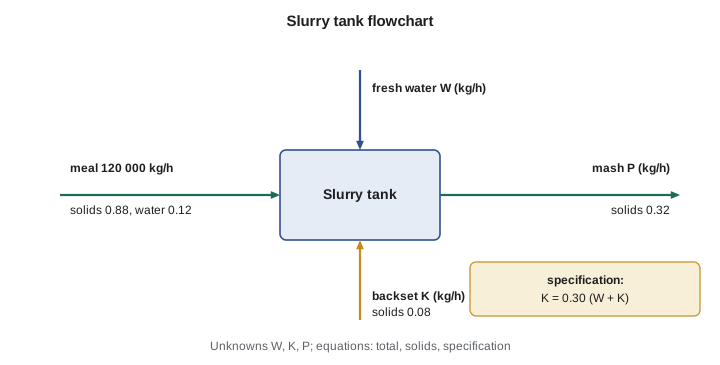
Meal at 120 000 kg/h contains 88 percent solids; the remainder is water. Backset contains 8 percent solids. The mash leaving the slurry tank must be 32 percent solids, and the backset flow \(K\) must be 30 percent of the total liquid added, \(K = 0.30(W + K)\), where \(W\) is fresh water. Find \(W\), \(K\) and the mash flow \(P\).
Show solution
- Unknowns: \(W, K, P\) (three). Equations: total balance, solids balance, backset rule (three). Degrees of freedom \(= 0\).
- Total: \(120\,000 + W + K = P\). Solids: \(0.88(120\,000) + 0.08K = 0.32P\). Rule: \(0.70K = 0.30W\), so \(W = 2.333K\).
- Substitute into the total balance: \(P = 120\,000 + 3.333K\). Then the solids balance gives \(105\,600 + 0.08K = 38\,400 + 1.0667K\), so \(K = 68\,110\ \text{kg/h}\).
- \(W = 158\,920\ \text{kg/h}\) and \(P = 347\,030\ \text{kg/h}\).
- Check: solids out \(= 0.32 \times 347\,030 = 111\,050\); solids in \(= 105\,600 + 5450 = 111\,050\ \text{kg/h}\).
Answer: The tank needs about 159 t/h of fresh water and 68 t/h of backset and produces 347 t/h of mash. Recycling backset saves fresh water and returns nutrients for the yeast, which is why every dry-grind plant does it.
Look at how the order of solution was chosen. The specification related only two unknowns, so it was used first to eliminate one; the total balance then expressed \(P\) in terms of \(K\); and the solids balance gave a single equation in \(K\). Looking for an equation with only one unknown, or a set of equations that can be solved together, is the main skill in hand solution. When the equations do not separate neatly, treat them as a linear system and solve them all at once.
Balances as linear systems
Material balances on nonreacting systems with known compositions are linear in the flow rates. Writing them in matrix form, \(\mathbf{A}\mathbf{x} = \mathbf{b}\), turns any balance problem into a standard calculation that a spreadsheet, a calculator or a few lines of code can solve. Process simulators build and solve systems with thousands of such equations. The program below solves the slurry tank and a beer column split with a small Gaussian elimination routine, so you can see exactly what the computer does.
# Solving material balance equations as a linear system (no libraries needed)

def solve(A, b):
    """Gaussian elimination with partial pivoting. A is a list of rows, b a list."""
    n = len(b)
    M = [row[:] + [bi] for row, bi in zip(A, b)]
    for c in range(n):
        p = max(range(c, n), key=lambda r: abs(M[r][c]))
        M[c], M[p] = M[p], M[c]
        for r in range(c + 1, n):
            f = M[r][c] / M[c][c]
            for k in range(c, n + 1):
                M[r][k] -= f * M[c][k]
    x = [0.0] * n
    for r in range(n - 1, -1, -1):
        x[r] = (M[r][n] - sum(M[r][k] * x[k] for k in range(r + 1, n))) / M[r][r]
    return x

# 1. Slurry tank: meal (88 % solids) + fresh water + backset (8 % solids) -> mash at 32 % solids
#    Unknowns: water W and backset K (kg/h); meal fixed at 120 000 kg/h; backset is 30 % of the liquid added.
meal, s_meal, s_back, s_mash = 120_000.0, 0.88, 0.08, 0.32
# total:  meal + W + K = P ; solids: s_meal*meal + s_back*K = s_mash*P ; backset rule: K = 0.30 (W + K)
# Unknowns ordered [W, K, P]
A = [[1, 1, -1],
     [0, s_back, -s_mash],
     [-0.30, 0.70, 0]]
b = [-meal, -s_meal * meal, 0]
W, K, P = solve(A, b)
print(f"Slurry tank: fresh water {W:9.0f} kg/h, backset {K:9.0f} kg/h, mash {P:9.0f} kg/h")

# 2. Beer column, two-component approximation: feed F at 13.5 % ethanol
F, zF = 280_000.0, 0.135
xD, xB = 0.58, 0.0005        # ethanol mass fractions in overhead vapour and bottoms
A = [[1, 1], [xD, xB]]       # unknowns [D, B]
D, B = solve(A, [F, zF * F])
rec = xD * D / (zF * F)
print(f"Beer column: overhead {D:9.0f} kg/h, bottoms {B:9.0f} kg/h, ethanol recovery {rec * 100:.2f} %")Slurry tank: fresh water 158919 kg/h, backset 68108 kg/h, mash 347027 kg/h Beer column: overhead 64987 kg/h, bottoms 215013 kg/h, ethanol recovery 99.72 %
Separation units and recovery
Separation units split one stream into two or more of different composition. For a two-component separation with a feed \(F\) of mass fraction \(z_F\), a top product \(D\) of fraction \(x_D\) and a bottom product \(B\) of fraction \(x_B\), the total and component balances give the product flows directly. The fractional recovery of a component is the fraction of its feed that leaves in the desired product.
Worked problem
Splitting the beer
Beer at 280 000 kg/h contains 13.5 percent ethanol by mass; treat it as ethanol and water. The beer column sends a vapour of 58 percent ethanol to the rectifier and leaves whole stillage containing 0.05 percent ethanol at the bottom. Find the overhead and bottoms flows and the ethanol recovery.
Show solution
- Unknowns \(D, B\); two balances; degrees of freedom \(= 0\).
- \(D = 280\,000(0.135 - 0.0005)/(0.58 - 0.0005) = 64\,990\ \text{kg/h}\).
- \(B = 280\,000 - 64\,990 = 215\,010\ \text{kg/h}\).
- Recovery \(= 0.58 \times 64\,990/(0.135 \times 280\,000) = 0.9972\).
Answer: The column recovers 99.7 percent of the ethanol. The 0.3 percent lost in the stillage, about 108 kg/h, is worth roughly a million dollars a year, which is why plants watch the bottoms analysis closely. Real beer also contains dissolved and suspended solids that all leave in the stillage; adding them as a third component changes the flows but not the method.
Tie components and scaling
A tie component is a material that passes from one stream to another unchanged, such as an inert solid in a dryer or nitrogen in a combustion gas. A balance on a tie component often gives a ratio between two streams in one step. In a dryer, the dry solids leaving equal the dry solids entering, which links the wet feed and the dried product immediately.
Because nonreacting balances are linear and homogeneous in the flows, a solution on any basis can be scaled. If 100 kg of feed gives 23.2 kg of overhead, then 280 000 kg/h of feed gives 64 990 kg/h. Scaling multiplies every flow by the same factor but leaves every fraction and ratio unchanged. This is why the choice of basis is free, and why engineers often solve on 100 kg or 100 mol and scale at the end.
When the data do not agree
Plant problems are often overspecified. Suppose the meal flowmeter, the fresh water meter, the backset meter and the mash meter all report values, and the laboratory measures the solids in each stream. That is four measured flows for three unknowns, so the degrees of freedom are negative, and the measurements are very unlikely to satisfy every balance exactly. Theo finds that the measured mash flow is 2.1 percent higher than the sum of the three inlet meters. Ingrid does not average the numbers or pick the one she likes. She first checks which meters were calibrated recently, then uses the solids balance as an independent check: if the solids balance closes with the inlet meters but not with the mash meter, the mash meter is the likely culprit.
This habit, using the redundancy in overspecified data to find bad measurements, is one of the most practical uses of balances in operating plants. More formal methods, called data reconciliation, adjust every measurement by the smallest amount consistent with its accuracy so that all balances close, and they flag measurements that need large adjustments as probably faulty. Every major plant historian and simulator offers some form of it.
Choosing the system boundary
A balance can be written around any boundary: a single unit, a junction where streams meet, a group of units, or the whole process. Each boundary gives its own set of independent equations, but the sets overlap: for a process of several units, the balances on all the individual units together contain the same information as the balances on all but one unit plus the overall balance. A useful strategy is to start with the boundary that has zero degrees of freedom, solve it, and carry the results into the next boundary. Lesson 4 develops this for multiple-unit processes, where choosing the right order can turn a tangle of equations into a sequence of easy steps.
Common mistakes
MistakeWriting a total balance and all N species balances and counting them as N + 1 equations.
InsteadOnly N are independent; the total balance is the sum of the species balances.
MistakeCounting each fraction in a stream as a separate unknown.
InsteadFractions sum to one; label all but one and get the last by difference.
MistakeStarting algebra before counting degrees of freedom.
InsteadCount first; a problem with positive degrees of freedom has no unique answer.
MistakeIgnoring a process specification such as a recycle ratio.
InsteadSpecifications are equations too and must be counted and used.
MistakeScaling fractions along with flows.
InsteadScaling changes flows only; compositions stay the same.
Summary and key terms
- Follow a standard procedure: label, basis, convert, count, write, solve, check.
- For N nonreacting species, at most N independent balances can be written for each system.
- Other equations come from specifications, physical relations and constraints.
- Degrees of freedom = unknowns − independent equations; it must be zero to solve.
- Nonreacting balances are linear and can be solved as A x = b and scaled freely.
- Recovery is the fraction of a component's feed that leaves in the desired product.
- Degrees of freedom
- The number of unknowns minus the number of independent equations.
- Underspecified
- Having more unknowns than independent equations.
- Overspecified
- Having more independent equations than unknowns.
- Process specification
- A stated fact about a process, such as a ratio, recovery or split.
- Tie component
- A material that passes between streams unchanged, linking their flows.
- Fractional recovery
- The fraction of a component in the feed that leaves in a chosen product.
- Backset
- Thin stillage recycled to the front of an ethanol plant to make up mash liquid.
Practice problems
Work each problem on paper first, then reveal the answer to check.
A mixer combines two streams of known composition into one unknown stream with three components. Count the degrees of freedom if both feed flows are known.
Show answer
Unknowns: product flow and two independent fractions (3); balances: 3; DF = 0.
Write the solids balance for a dryer fed 1000 kg/h of grains at 35 % solids that produces grains at 90 % solids.
Show answer
0.35(1000) = 0.90 P, so P = 389 kg/h and 611 kg/h of water evaporates.
A column feed is 40 % A; top product 95 % A; bottoms 2 % A; feed 100 kmol/h. Find the top product flow.
Show answer
D = 100(0.40 − 0.02)/(0.95 − 0.02) = 40.9 kmol/h.
Why is a problem with negative degrees of freedom useful with plant data?
Show answer
The extra measurements can be checked against each other to detect errors.
In the program, raise the target mash solids to 0.34. What happens to the fresh water?
Show answer
Fresh water falls to about 143 500 kg/h because less liquid is needed.
What recovery does the beer column achieve if the bottoms ethanol rises to 0.2 %?
Show answer
D = 280 000(0.133)/0.578 = 64 430 kg/h; recovery = 0.58 × 64 430/37 800 = 98.9 %.
Lesson quiz · 5 questions
Score 60% or more to complete this lesson.
Create a free account to save your progress, take quizzes and earn a certificate.