Evaluating models: accuracy, precision, recall and more

The first no-show model came back from training with a headline number: 92 correct predictions out of every 100 on the test set. Jonah was ready to celebrate. Noor wrote another number beside it: 94. "That," she said, "is the accuracy of a model that predicts nobody will ever miss an appointment. Our model is worse than doing nothing, if accuracy is all we look at."

This lesson explains why. It covers the confusion matrix and the metrics built from it, the metrics for regression, and the business metrics that decide whether a model is worth using at all.

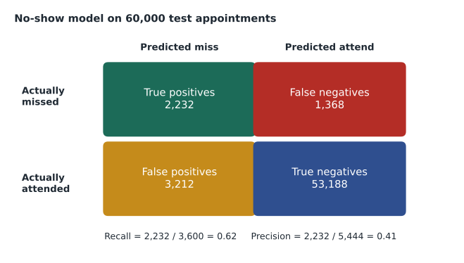
The confusion matrix

For a classification model, every prediction falls into one of four boxes. Using the no-show model, where the "positive" class is a missed appointment:

• True positive (TP): predicted a miss, and the client did miss. 2,232 appointments.
• False positive (FP): predicted a miss, but the client came. 3,212 appointments. These clients receive an unnecessary extra reminder.
• False negative (FN): predicted the client would come, but they missed. 1,368 appointments. These are the misses the model failed to catch.
• True negative (TN): predicted the client would come, and they did. 53,188 appointments.

The test set held 60,000 appointments from the six months to September 2026, of which 3,600, or 6 in every 100, were missed. Laying the results out this way, in a confusion matrix, makes it obvious that the model's errors come in two kinds with different costs.

Accuracy and its trap

Accuracy is the share of all predictions that were correct: (TP + TN) divided by the total. For the no-show model that is (2,232 + 53,188) ÷ 60,000, about 0.924. It sounds good, but the classes are imbalanced: 94 of every 100 appointments are kept. A useless model that always predicts "will attend" scores 0.94 accuracy and catches no misses at all. Whenever one class is rare, accuracy hides the very thing you care about.

Precision, recall and F1

Two metrics look at the positive class directly.

• Precision answers: of the appointments the model flagged, how many were really missed? TP ÷ (TP + FP) = 2,232 ÷ 5,444 ≈ 0.41. About 4 of every 10 flagged clients would have missed.
• Recall (also called sensitivity or true positive rate) answers: of all the appointments that were missed, how many did the model catch? TP ÷ (TP + FN) = 2,232 ÷ 3,600 = 0.62.

Precision and recall pull against each other. A model usually outputs a probability, and a threshold turns it into a yes or no. Lower the threshold and the model flags more bookings: recall rises, because more misses are caught, but precision falls, because more of the flagged clients would have come anyway. Raise it and the reverse happens. Which matters more depends on the cost of each error. For the no-show pilot, a false positive costs one friendly extra reminder, while a false negative costs an empty appointment slot, so Andre preferred higher recall. For a model that decided to cancel a booking, a false positive would be unacceptable, which is one reason the company will never use the model that way.

The F1 score combines the two into one number: the harmonic mean, 2 × precision × recall ÷ (precision + recall). For the no-show model it is about 0.49. F1 is useful for comparing models on imbalanced data, but it treats both errors as equally bad, which is rarely true in business.

Curves and AUC

Because every threshold gives a different precision and recall, it helps to look at all of them at once. The ROC curve plots the true positive rate (recall) against the false positive rate, FP ÷ (FP + TN), as the threshold moves. The area under the curve (AUC) summarizes it in one number between 0.5, no better than chance, and 1.0, perfect ranking. AUC measures how well a model ranks positives above negatives regardless of threshold, so it is handy for comparing models before choosing a threshold. The no-show model's AUC on the test set was 0.81.

Metrics for regression

Regression models predict numbers, so they are judged by how far predictions are from the truth.

• Mean absolute error (MAE): the average size of the errors, in the original units. A visit-length model with an MAE of 6 minutes is off by 6 minutes on average.
• Root mean squared error (RMSE): the square root of the average squared error. Squaring punishes large errors more, so RMSE is higher than MAE when a few predictions are badly wrong.
• R-squared (R²): the share of the variation in the target that the model explains, from 0 to 1 for useful models. 0.7 means the model explains about 70 out of every 100 units of variation around the average.

Business metrics

A model can have excellent technical metrics and still not be worth running. The exam guide lists business measures that belong beside them: cost per user or per prediction, development costs, customer feedback, and return on investment (ROI), the benefit gained compared with the cost. For the no-show pilot, Lorraine Beaudry wanted a simple calculation before she would approve it.

# Model metrics and a simple business case for the no-show pilot.
TP, FP, FN, TN = 2232, 3212, 1368, 53188
total = TP + FP + FN + TN

accuracy = (TP + TN) / total
precision = TP / (TP + FP)
recall = TP / (TP + FN)
f1 = 2 * precision * recall / (precision + recall)
always_attend = (FP + TN) / total          # baseline: predict nobody misses
print("accuracy", round(accuracy, 3), "| baseline accuracy", round(always_attend, 3))
print("precision", round(precision, 2), "| recall", round(recall, 2), "| F1", round(f1, 2))

# Business view over the six-month test period (illustrative figures).
reminder_cost = 2.0        # dollars per extra reminder call or text
slot_value = 120.0         # dollars of revenue per kept appointment slot
saved_share = 0.25         # assume 1 in 4 caught misses is rescued by the reminder
cost = (TP + FP) * reminder_cost
benefit = TP * saved_share * slot_value
print("extra reminders cost", round(cost), "dollars; recovered slots worth", round(benefit), "dollars")
print("return per dollar spent:", round(benefit / cost, 1))

accuracy 0.924 | baseline accuracy 0.94
precision 0.41 | recall 0.62 | F1 0.49
extra reminders cost 10888 dollars; recovered slots worth 66960 dollars
return per dollar spent: 6.1

The technical metrics confirm that accuracy is the wrong yardstick here. The business view is what persuaded Lorraine: even assuming only one in four caught misses is rescued, and with the illustrative prices labelled as such, the extra reminders return several dollars for each dollar spent. The assumption about rescued slots is the weakest number, so the pilot was designed to measure it directly, as lesson 12 describes.

Metrics for other kinds of AI

Other tasks have their own yardsticks, and the exam may mention them by name. Speech recognition is often judged by word error rate, the share of words wrongly substituted, missed or inserted compared with a human transcript. Object detection in images uses intersection over union, how much a predicted box overlaps the true one. Generative text is harder to score automatically; metrics such as BLEU and ROUGE compare generated text with reference text by counting overlapping words, and they are often paired with human review. AWS-113 covers evaluating foundation model output in depth. The common thread is that every metric simplifies, so it should be chosen to match the decision the model supports and checked against human judgement.

Evaluating by group

Hannah asked a question that every evaluation should include: does the model perform equally well for different groups? Noor broke the test results down by clinic. Recall ranged from 0.55 at the Kelowna clinic to 0.68 in Calgary. The gap was explained by fewer reminder confirmations being recorded at the smaller clinic, which was a data problem, not a reason to treat its clients differently. Checking metrics by group, not only overall, is the first practical step toward the fairness work in AWS-114, and SageMaker Clarify, met in lesson 9, automates many of these checks.

Choosing the threshold with the business

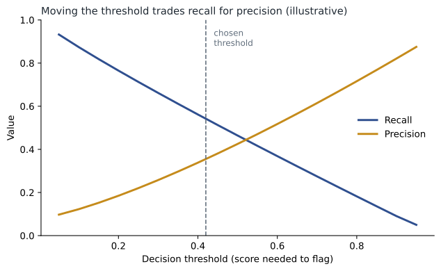
Because precision and recall trade off, the threshold is a business decision, not a technical one. Noor showed Andre a small table of options from the validation data: at a strict threshold the model flagged about 2,500 bookings a month at the six pilot clinics, with high precision and recall near 0.45; at the chosen threshold it flagged about 5,400, with recall 0.62; at a loose threshold it flagged over 9,000, with recall near 0.80 but more than two false alarms for every real miss. Andre asked how many extra reminders the front desks could realistically send each evening. The answer, about 60 per clinic, fixed the threshold. This is typical: the right operating point comes from the capacity and costs of the people acting on the predictions, and it should be revisited when those change.

Precision and recall in other settings

Different problems weigh the two errors very differently, and exam questions often describe the costs and expect you to pick the metric. In medical screening, missing a disease is usually worse than a false alarm that leads to a follow-up test, so recall matters most. In spam filtering, sending a genuine email to the spam folder is worse than letting an occasional spam through, so precision matters more. In fraud detection, both errors are costly, and teams often track both along with the money involved. For the no-show pilot the balance favoured recall, because a false alarm costs a courteous message. A useful exercise for any classifier is to write one sentence for each error: what happens to a person when the model is wrong in this way? The answers usually show which metric to optimize and where to set the threshold.

Another common metric is specificity, the share of true negatives correctly identified, TN ÷ (TN + FP). For the no-show model it is 53,188 ÷ 56,400, about 0.94: most clients who would attend are correctly left off the list. Specificity and recall together describe how a model treats each class.

Jonah's own summary, written on a sticky note above his desk, read: accuracy only beside its baseline; precision for "how many flags were right"; recall for "how many real cases we caught"; the threshold set by what people can act on; and a business number, in dollars or hours, beside every technical one. He found that most practice questions in this domain could be answered with that note alone.