
AI-470 · Lesson 4 of 12 · 23 min
Decisions under uncertainty: utility and Markov decision processes
Real agents rarely know exactly what their actions will do. A delivery drone may be pushed by wind; a sales email may or may not get a reply; an API call may time out; a robot's grasp may slip. Goal-based planning that assumes deterministic outcomes breaks down. Decision theory provides the framework for acting well under uncertainty: assign utilities to outcomes, weigh them by their probabilities, and choose actions that maximize expected utility. For sequential decisions, where each action changes the situation for the next, Markov decision processes (MDPs) extend this to policies that specify what to do in every state. This lesson covers expected utility, MDPs, value iteration and policy iteration, discounting, partially observable problems, and how these ideas inform the design of modern agents.
Expected utility
A utility function assigns a number to each outcome, representing how desirable it is to the agent or its principal. When an action \(a\) can lead to outcomes \(s'\) with probabilities \(P(s' \mid a)\), its expected utility is:
A rational agent chooses the action with the highest expected utility. This simple principle handles trade-offs that goal-based agents cannot express: a fast route with a small chance of a long delay against a slower reliable route, or an action that usually succeeds cheaply but occasionally causes a costly failure. Utilities need not be money; they can combine time, cost, risk, quality and user satisfaction. Choosing them carefully is important, because an agent will faithfully optimize whatever it is given, including flaws in the utility function.
Worked problem
Choosing an action by expected utility
A support agent can either answer a customer question immediately (80 % chance the answer is right, utility +10; 20 % chance it is wrong, utility −30) or first check the knowledge base, which costs time (utility −2) and raises the chance of a correct answer to 97 %. Which action has higher expected utility?
Show solution
- Answer immediately: 0.8 × 10 + 0.2 × (−30) = 8 − 6 = 2.
- Check first: −2 + 0.97 × 10 + 0.03 × (−30) = −2 + 9.7 − 0.9 = 6.8.
- Checking first has higher expected utility (6.8 against 2).
- If wrong answers cost only −5, answering immediately would give 0.8 × 10 + 0.2 × (−5) = 7, beating 6.8.
- The best action depends on how costly errors are, which is why utility design matters.
Answer: Check the knowledge base first (6.8 against 2), unless wrong answers are cheap.
Markov decision processes
An MDP models sequential decisions with uncertain outcomes. It consists of:
- A set of states \(S\) and actions \(A\).
- A transition model \(P(s' \mid s, a)\), the probability of reaching state \(s'\) after taking action \(a\) in state \(s\).
- A reward function \(R(s, a, s')\) giving immediate rewards or costs.
- A discount factor \(\gamma\) between 0 and 1 that weights future rewards less than immediate ones.
The Markov property states that the future depends only on the current state and action, not on the history of how the agent got there; if history matters, it must be included in the state. A solution to an MDP is a policy \(\pi(s)\), specifying an action for every state, rather than a fixed plan. Because outcomes are uncertain, the agent may end up anywhere, and a policy tells it what to do wherever it finds itself.
Value functions and the Bellman equation
The value \(V(s)\) of a state under the optimal policy is the expected discounted sum of rewards starting there and acting optimally. It satisfies the Bellman optimality equation, which says that a state's value is the best achievable combination of immediate reward and discounted value of where you end up:
Value iteration solves this equation by starting with arbitrary values and repeatedly applying it as an update to every state until the values stop changing. The optimal policy then picks, in each state, the action that achieves the maximum. Policy iteration alternates between evaluating the current policy and improving it greedily, and often converges in fewer iterations. Both are guaranteed to find the optimal policy for finite MDPs with \(\gamma < 1\).
import numpy as np
# Value iteration for a robot in a 4 x 4 grid with a slippery floor
n, gamma, slip = 4, 0.95, 0.2
reward = np.full((n, n), -0.04); reward[0, 3] = 1.0; reward[1, 3] = -1.0
terminal = {(0, 3), (1, 3)}; wall = {(1, 1)}
acts = {"up": (-1, 0), "down": (1, 0), "left": (0, -1), "right": (0, 1)}
def step(s, a):
    r, c = s[0] + acts[a][0], s[1] + acts[a][1]
    if not (0 <= r < n and 0 <= c < n) or (r, c) in wall:
        return s
    return (r, c)
side = {"up": ("left", "right"), "down": ("left", "right"), "left": ("up", "down"), "right": ("up", "down")}
V = np.zeros((n, n))
for it in range(200):
    newV = V.copy()
    for r in range(n):
        for c in range(n):
            s = (r, c)
            if s in terminal or s in wall:
                newV[s] = reward[s] if s in terminal else 0
                continue
            best = -1e9
            for a in acts:
                outcomes = [(1 - slip, step(s, a))] + [(slip / 2, step(s, b)) for b in side[a]]
                best = max(best, sum(p * (reward[s] + gamma * V[t]) for p, t in outcomes))
            newV[s] = best
    delta = np.abs(newV - V).max(); V = newV
    if delta < 1e-6:
        break
print(f"converged after {it + 1} sweeps")
arrow = {"up": "^", "down": "v", "left": "<", "right": ">"}
for r in range(n):
    row_v, row_p = [], []
    for c in range(n):
        s = (r, c)
        row_v.append(f"{V[s]:6.2f}")
        if s in terminal:
            row_p.append("+" if reward[s] > 0 else "-")
        elif s in wall:
            row_p.append("#")
        else:
            q = {a: sum(p * V[t] for p, t in [(1 - slip, step(s, a))] + [(slip / 2, step(s, b)) for b in side[a]]) for a in acts}
            row_p.append(arrow[max(q, key=q.get)])
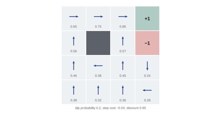
print(" ".join(row_v), " ", " ".join(row_p))converged after 33 sweeps 0.65 0.75 0.86 1.00 > > > + 0.56 0.00 0.57 -1.00 ^ # ^ - 0.46 0.38 0.45 0.24 ^ < ^ v 0.38 0.32 0.36 0.28 ^ ^ ^ <
Values converge after 33 sweeps. The robot gets −0.04 per step to encourage short paths, +1 for reaching the goal at the top right and −1 for the hazard just below it, and the floor is slippery: 20 % of the time it slides sideways. The policy arrows head toward the goal, but notice the cell just below the hazard: its best action is to move down, away from both, because moving up risks sliding into the hazard. The bottom-right cell moves left for the same reason. The optimal policy balances reward against risk automatically, and changing the slip probability, step cost or discount changes how cautious it is, which is a concrete illustration of how utility design shapes behaviour.
Discounting and horizons
The discount factor expresses how much the agent values future rewards. With \(\gamma = 0.9\), a reward ten steps away is worth \(0.9^{10} \approx 0.35\) of an immediate one; with \(\gamma = 0.99\), it is worth about 0.90. Discounting reflects uncertainty about the future, the preference for earlier results, and ensures that infinite sums of rewards remain finite. Low discount factors produce short-sighted agents; high ones produce far-sighted agents that are harder to train. Some problems instead have a finite horizon, such as a fixed number of steps or a deadline, where the optimal policy can depend on how much time remains.
Partial observability
Many agents cannot observe the full state. A robot is uncertain of its position; a dialogue agent does not know exactly what the user wants; a diagnostic agent cannot see the underlying fault. Partially observable MDPs (POMDPs) model this with observation probabilities, and the agent maintains a belief state, a probability distribution over possible states, updated by Bayes' rule after each action and observation (as in the localization filters of AI-450). The optimal policy maps belief states to actions, and it naturally values information-gathering actions, such as asking a clarifying question or running a diagnostic test, because they sharpen the belief and lead to better decisions later. Exact POMDP solutions are intractable for large problems, but approximate methods and the principle of acting on beliefs are widely used.
The value of information
Decision theory quantifies when gathering information is worthwhile. The value of perfect information is the improvement in expected utility from knowing an uncertain quantity before deciding, compared with deciding now. If it exceeds the cost of obtaining the information, the agent should seek it. A language model agent deciding whether to ask the user a clarifying question, search the documentation, or run a test before acting faces exactly this trade-off: asking costs the user time, but acting on a wrong assumption may cost much more. Good agents ask when uncertainty is high and stakes are significant, and proceed when the answer would not change what they do.
From MDPs to modern agents
Few practical agents explicitly solve MDPs, because their state spaces are huge and their transition models unknown. Yet the framework shapes how we think about them. Reinforcement learning (Lesson 5) learns policies and values from experience when the model is unknown. Language model agents are trained with reinforcement learning on rewards from task success and human or model feedback. And design questions, such as what the reward should be, how to trade speed against reliability, when to gather information and how to handle uncertainty, are MDP questions in everyday clothing.
| Concept | Classical meaning | Modern agent analogue |
|---|---|---|
| State | Complete description of the situation | Conversation, files, tool results, memory |
| Action | Choice from a defined set | Tool call, message, file edit |
| Transition model | Probabilities of next states | How the environment responds to actions |
| Reward | Immediate payoff | Task success, user feedback, cost |
| Policy | Action for every state | The model's behaviour given its context |
| Belief state | Distribution over hidden states | Uncertainty about user intent or system state |
Risk attitudes and utility shape
Expected utility can represent different attitudes to risk through the shape of the utility function. A risk-neutral agent values outcomes linearly, caring only about averages. A risk-averse agent has a concave utility, valuing a sure outcome more than a gamble with the same average, which is appropriate when large losses would be catastrophic, such as an agent managing a company's cash or controlling physical equipment. Designers can also impose explicit constraints, such as keeping the probability of a severe failure below a threshold, rather than relying only on averages. For agents acting on behalf of people, matching the principal's risk attitude, which is often more cautious than a simple average suggests, is part of aligning behaviour with intent.
Finally, decisions under uncertainty benefit from honest probabilities. An agent that is overconfident, treating a 60 % guess as a near certainty, will skip checks and take risks it should avoid, while a well-calibrated agent knows when to gather more information. Calibration of model confidence is therefore part of good decision making.
Many everyday agent decisions are small expected-utility calculations in disguise: whether to run the full test suite or just one test, whether to search again or answer now, whether to retry a failed call or report it. Making these trade-offs explicit, even roughly, leads to agents that are faster when stakes are low and more careful when stakes are high.
Common mistakes
MistakeAssuming actions always succeed.
InsteadModel outcome probabilities and plan for failures.
MistakeProducing a fixed plan for an uncertain world.
InsteadUse a policy that says what to do in any state.
MistakeDesigning rewards without considering side effects.
InsteadCheck what behaviour the reward actually encourages.
MistakeNever gathering information before acting.
InsteadWeigh the value of information against its cost.
MistakeLeaving relevant history out of the state.
InsteadInclude what matters so the Markov property holds.
Summary and key terms
- Rational agents maximize expected utility under uncertainty.
- MDPs have states, actions, transitions, rewards and a discount factor.
- Policies map every state to an action.
- The Bellman equation defines optimal values; value iteration solves it.
- Discount factors control how far-sighted the agent is.
- POMDPs act on belief states and value information gathering.
- MDP concepts guide reward design and behaviour of modern agents.
- Utility
- Numerical desirability of an outcome.
- Expected utility
- Probability-weighted average utility.
- MDP
- Markov decision process.
- Markov property
- Future depends only on the present state and action.
- Policy
- Mapping from states to actions.
- Value function
- Expected discounted return from a state.
- Bellman equation
- Recursive definition of optimal values.
- Discount factor
- Weight applied to future rewards.
- POMDP
- MDP with partial observations.
- Value of information
- Gain from knowing something before deciding.
Practice problems
Work each problem on paper first, then reveal the answer to check.
Compute EU for outcomes +20 (0.6) and −10 (0.4).
Show answer
12 − 4 = 8.
List the components of an MDP.
Show answer
States, actions, transitions, rewards, discount.
What is the Markov property?
Show answer
The future depends only on the current state and action.
Why is an MDP solution a policy rather than a plan?
Show answer
Outcomes are uncertain, so the agent may be anywhere.
What does value iteration repeat?
Show answer
Bellman updates for all states until convergence.
In C4, why does the cell below the hazard move down?
Show answer
Moving up risks sliding into the hazard.
Value of a reward 5 steps away with γ = 0.8?
Show answer
0.8⁵ ≈ 0.33.
What is a belief state?
Show answer
A probability distribution over possible states.
When should an agent ask a clarifying question?
Show answer
When the information is worth more than its cost.
What learns policies when the model is unknown?
Show answer
Reinforcement learning.
Lesson quiz · 5 questions
Score 60% or more to complete this lesson.
Create a free account to save your progress, take quizzes and earn a certificate.