
AI-470 · Lesson 2 of 12 · 24 min
Search: how goal-based agents find their way
A goal-based agent must work out a sequence of actions that leads from where it is to where it wants to be. When the environment is known, observable and deterministic, this is a search problem: explore the space of possible states, following the actions that connect them, until a goal state is found. Search underlies route planners, puzzle solvers, game-playing programs, robot motion planning and the scheduling of many industrial systems, and its ideas, frontiers, heuristics and the trade-off between exploring broadly and pursuing promising paths, reappear in planning with language models. This lesson formulates search problems, compares uninformed and informed search algorithms, explains heuristics and A*, and introduces local search and adversarial search for games.
Formulating a search problem
A search problem has five components:
- An initial state, such as the robot's starting cell.
- Actions available in each state, such as moving north, south, east or west.
- A transition model describing the state that results from each action.
- A goal test, which checks whether a state is a goal.
- A path cost, the sum of action costs, such as distance travelled or time taken.
The states and transitions form a state space graph. A solution is a path from the initial state to a goal; an optimal solution has the lowest path cost. Choosing the right abstraction is crucial: a delivery robot planning a route across a city does not need to represent every wheel rotation, only intersections and roads, while a motion planner for its arm needs continuous joint angles. Good abstractions make problems small enough to solve while keeping the details that matter.
Uninformed search
Uninformed search algorithms use no knowledge about where the goal is. They differ in the order in which they expand states from the frontier, the set of discovered but unexpanded states:
- Breadth-first search (BFS) expands the shallowest states first, using a queue. It finds the path with the fewest steps and is optimal when all actions cost the same, but its memory use grows exponentially with depth.
- Uniform-cost search (Dijkstra's algorithm) expands the state with the lowest path cost so far, using a priority queue. It is optimal for any non-negative action costs.
- Depth-first search (DFS) expands the deepest state first, using a stack. It uses little memory but can wander down long or infinite paths and is not optimal.
- Iterative deepening runs depth-limited DFS with increasing limits, combining the low memory of DFS with the completeness and optimality (for equal costs) of BFS.
Search algorithms keep track of states already reached, so they do not expand the same state repeatedly, which is essential in graphs with cycles.
| Algorithm | Frontier | Complete? | Optimal? | Memory |
|---|---|---|---|---|
| Breadth-first | Queue | Yes | Yes, for equal costs | High (exponential in depth) |
| Uniform-cost | Priority by path cost | Yes | Yes | High |
| Depth-first | Stack | Not in infinite spaces | No | Low (linear in depth) |
| Iterative deepening | Repeated depth-limited stacks | Yes | Yes, for equal costs | Low |
| Greedy best-first | Priority by heuristic | Not always | No | High |
| A* | Priority by cost + heuristic | Yes | Yes, with admissible heuristic | High |
Heuristics and A*
Informed search uses a heuristic \(h(n)\), an estimate of the cost from state \(n\) to the nearest goal. Greedy best-first search expands the state with the smallest \(h\), heading straight for the goal, which is often fast but can be misled into long detours. A* search combines the cost so far \(g(n)\) with the heuristic:
A* expands the state with the lowest \(f\), the estimated total cost of the best path through it. If the heuristic is admissible, never overestimating the true remaining cost, A* is guaranteed to find an optimal path. If it is also consistent, meaning the estimate never drops by more than the cost of a single step, A* never needs to re-expand a state. On a grid where movement is in four directions with unit cost, the Manhattan distance, the sum of horizontal and vertical distances to the goal, is admissible and consistent; straight-line distance is admissible for road maps.
import numpy as np
import heapq
# A* search for a delivery robot on a grid with obstacles
grid = np.zeros((12, 16), int)
grid[2:10, 5] = 1; grid[2, 5:12] = 1; grid[6:12, 10] = 1; grid[0:5, 13] = 1
start, goal = (11, 0), (0, 15)
def neighbors(p):
    r, c = p
    for dr, dc in ((1, 0), (-1, 0), (0, 1), (0, -1)):
        q = (r + dr, c + dc)
        if 0 <= q[0] < 12 and 0 <= q[1] < 16 and grid[q] == 0:
            yield q
def search(use_heuristic):
    h = (lambda p: abs(p[0] - goal[0]) + abs(p[1] - goal[1])) if use_heuristic else (lambda p: 0)
    frontier = [(h(start), 0, start)]; came = {start: None}; cost = {start: 0}; expanded = 0
    while frontier:
        _, g, p = heapq.heappop(frontier)
        if g > cost[p]:
            continue
        expanded += 1
        if p == goal:
            break
        for q in neighbors(p):
            if q not in cost or g + 1 < cost[q]:
                cost[q] = g + 1; came[q] = p
                heapq.heappush(frontier, (g + 1 + h(q), g + 1, q))
    path = [goal]
    while came[path[-1]] is not None:
        path.append(came[path[-1]])
    return len(path) - 1, expanded, path[::-1]
for name, hflag in (("uniform cost (no heuristic)", False), ("A* with Manhattan distance", True)):
    length, expanded, path = search(hflag)
    print(f"{name:28s} path length {length}, nodes expanded {expanded}")
show = np.full(grid.shape, ".")
show[grid == 1] = "#"
for p in path:
    show[p] = "*"
show[start] = "S"; show[goal] = "G"
print()
for row in show:
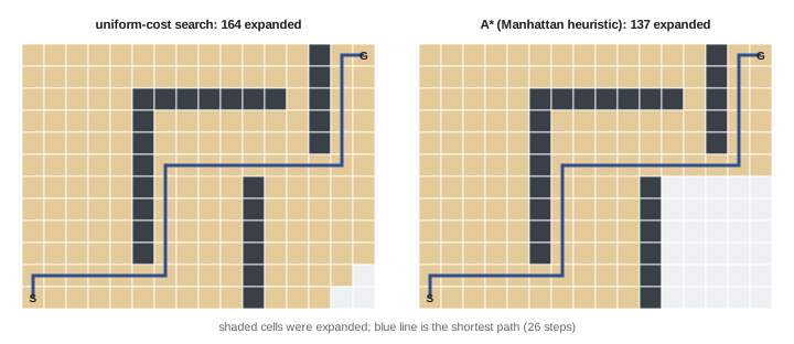
print("".join(row))uniform cost (no heuristic) path length 26, nodes expanded 164 A* with Manhattan distance path length 26, nodes expanded 137 .............#*G .............#*. .....#######.#*. .....#.......#*. .....#.......#*. .....#*********. .....#*...#..... .....#*...#..... .....#*...#..... .....#*...#..... *******...#..... S.........#.....
Both algorithms find a shortest path of 26 steps, shown with stars, but A* expands 137 states against 164 for uniform-cost search, because the heuristic steers it toward the goal. The saving here is modest because walls force a long detour that the heuristic cannot anticipate; in open spaces or larger maps, the savings are often dramatic. The quality of a heuristic is measured by how closely it approaches the true cost: the closer, the fewer states expanded. Heuristics can be designed by solving relaxed versions of the problem, for example ignoring walls, or learned from data, an approach used in modern planning systems and game-playing programs.
Local search and optimization
Some problems care only about the final state, not the path: scheduling, layout, configuration and parameter tuning. Local search algorithms keep one or a few current states and move to neighbouring states that improve an objective. Hill climbing always moves to a better neighbour and stops at a local optimum, which may not be the global best. Simulated annealing sometimes accepts worse moves, with a probability that decreases over time, to escape local optima. Genetic algorithms maintain a population of candidate solutions, combining and mutating them. Local search uses little memory and handles enormous spaces, at the cost of no guarantee of optimality. Many practical agent tasks, such as tuning a configuration or improving a draft, are local searches guided by feedback.
Adversarial search
When other agents act against you, as in chess or Go, search must consider their responses. Minimax search assumes the opponent plays optimally: the agent chooses the move that maximizes its minimum guaranteed outcome, alternating between maximizing and minimizing levels of a game tree. Alpha-beta pruning skips branches that cannot affect the decision, often allowing twice the search depth in the same time. Because full game trees are astronomically large, programs search to a limited depth and evaluate positions with a heuristic evaluation function. Monte Carlo tree search (MCTS) instead estimates the value of moves by simulating many games, focusing simulations on promising moves using a balance of exploitation and exploration. Combined with deep neural networks that evaluate positions and suggest moves, MCTS powered AlphaGo and AlphaZero, which defeated the best human players at Go and taught themselves chess and shogi from scratch.
Search inside modern agents
Search ideas appear throughout language model agents. Tree of Thoughts and related methods have the model propose several possible next steps, evaluate them and explore the most promising, a form of best-first or beam search over reasoning steps. Agents solving coding tasks may generate several candidate patches and use tests as a goal test. Planning systems for robots use classical search over symbolic states with learned heuristics. The vocabulary of states, actions, goals, costs, heuristics and frontiers remains a powerful way to think about what an agent is doing and why it might fail: an agent that never revisits earlier choices is doing greedy search, and can get stuck in the same ways.
Worked problem
Checking heuristic admissibility
A robot moves on a grid in four directions at cost 1 per step, but can also use a teleporter that moves it anywhere at cost 3. Is Manhattan distance still admissible? Suggest an admissible heuristic.
Show solution
- Manhattan distance can be large, for example 20 steps between distant cells.
- With the teleporter, the true cost from any cell to the goal is at most 3 (teleport directly to the goal).
- So Manhattan distance can overestimate the true cost (20 > 3) and is no longer admissible.
- An admissible heuristic is h(n) = min(Manhattan distance, 3), which never exceeds the true cost.
- This heuristic is weaker but keeps A* optimal.
Answer: No; use min(Manhattan distance, 3) to keep the heuristic admissible.
Search in continuous and very large spaces
Grid and graph search assume discrete states, but many agent problems are continuous: a robot arm has joint angles, a drone has position and velocity, and a design has real-valued parameters. Continuous problems are made searchable by discretization (dividing space into a grid or lattice), by sampling-based planners such as probabilistic roadmaps and rapidly exploring random trees, which build graphs of randomly sampled feasible states (covered in AI-450), or by optimization methods that adjust continuous variables directly. For enormous discrete spaces, such as all possible programs or molecules, agents combine search with learned models that propose promising candidates, the strategy behind systems that discover algorithms or design proteins.
Search costs and anytime algorithms
Real agents have limited time and computation. Anytime algorithms return a reasonable answer quickly and improve it if given more time, which suits agents that must act on deadlines. Weighted A*, which inflates the heuristic to search more greedily, finds good but not necessarily optimal solutions much faster, with a bound on how far from optimal they can be. Bounded-suboptimal search lets designers trade quality for speed explicitly. Thinking about computation as a resource to be allocated, deciding how much to search before acting, is itself a decision problem, and modern language model agents face it when deciding how long to reason before answering.
Choosing an algorithm
In practice, the choice of search algorithm follows from the problem: breadth-first search for small unweighted problems, uniform-cost search when actions have different costs and no good heuristic exists, A* when an admissible heuristic is available, iterative deepening when memory is tight, and local search when only the final state matters. Measuring the number of states expanded, the time taken and the solution quality on representative problems confirms the choice.
Search also teaches humility about scale. Problems that look simple, such as scheduling a few dozen tasks or planning a route with several stops, can have more possible solutions than there are atoms in the universe. Good abstractions, heuristics and problem decompositions are what make such problems tractable, and recognizing when a problem is too large for exhaustive search is the first step to choosing a practical approach.
Common mistakes
MistakeUsing DFS when the shortest path is required.
InsteadUse BFS, uniform-cost search or A*.
MistakeUsing a heuristic that overestimates.
InsteadEnsure admissibility for optimal A* results.
MistakeForgetting to track visited states.
InsteadRecord reached states to avoid loops and repeats.
MistakeModelling too much detail.
InsteadChoose an abstraction that keeps only what matters.
MistakeTrusting hill climbing to find the global optimum.
InsteadUse restarts, annealing or population methods.
Summary and key terms
- Search problems have initial states, actions, transitions, goal tests and path costs.
- BFS, uniform-cost, DFS and iterative deepening are uninformed strategies.
- A* uses f = g + h and is optimal with an admissible heuristic.
- Better heuristics expand fewer states.
- Local search optimizes final states with little memory but no guarantee.
- Minimax, alpha-beta and MCTS handle adversarial games.
- Search concepts explain how language model agents explore and fail.
- State space
- All states reachable through actions.
- Frontier
- Discovered but unexpanded states.
- Breadth-first search
- Expands shallowest states first.
- Uniform-cost search
- Expands lowest-cost states first.
- Heuristic
- Estimate of remaining cost to a goal.
- Admissible
- Never overestimates the true cost.
- A*
- Search ordering by cost so far plus heuristic.
- Hill climbing
- Local search moving to better neighbours.
- Minimax
- Adversarial search assuming optimal opponents.
- Monte Carlo tree search
- Game search using simulated playouts.
Practice problems
Work each problem on paper first, then reveal the answer to check.
Name the five components of a search problem.
Show answer
Initial state, actions, transition model, goal test, path cost.
Which algorithm finds fewest-step paths with equal costs?
Show answer
Breadth-first search.
Why is DFS memory-efficient?
Show answer
It stores only the current path and siblings.
Write the A* evaluation function.
Show answer
f(n) = g(n) + h(n).
What makes a heuristic admissible?
Show answer
It never overestimates.
In C2, how many states did A* expand?
Show answer
137, versus 164 for uniform-cost.
Why was the saving modest in C2?
Show answer
Walls forced detours the heuristic could not foresee.
How does simulated annealing escape local optima?
Show answer
It sometimes accepts worse moves.
What does alpha-beta pruning do?
Show answer
Skips branches that cannot affect the decision.
How do Tree of Thoughts methods relate to search?
Show answer
They explore and evaluate alternative reasoning steps.
Lesson quiz · 5 questions
Score 60% or more to complete this lesson.
Create a free account to save your progress, take quizzes and earn a certificate.