
AI-460 · Lesson 8 of 12 · 25 min
Differential privacy
Lesson 7 showed that anonymization by removing or generalizing identifiers repeatedly fails against attackers with auxiliary information. Differential privacy, introduced by Cynthia Dwork, Frank McSherry, Kobbi Nissim and Adam Smith in 2006, takes a different approach. Instead of describing what released data should look like, it constrains how much any single person's data can affect the output of an analysis. The guarantee holds whatever the attacker knows, it composes predictably across many analyses, and it can be quantified with a single parameter. Differential privacy is now used by the US Census Bureau, by Apple and Google for telemetry, and in machine learning libraries. This lesson explains the definition, the basic mechanisms, sensitivity, composition and practical deployment.
The intuition
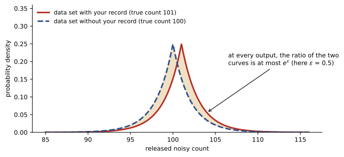
Imagine two worlds that differ only in whether your record is in a data set. An analysis is differentially private if its output is almost equally likely in both worlds. Then whatever an observer sees, they cannot be confident whether you participated, and so they learn very little that is specific to you. Crucially, the analysis can still reveal population-level facts: a differentially private study can show that smoking causes cancer, which tells an insurer something about smokers, but it would show that whether or not any particular smoker took part. Differential privacy protects individuals from harms caused by their participation, not from conclusions about groups.
The definition
Two data sets \(D\) and \(D'\) are neighbours if they differ in one person's record. A randomized mechanism \(M\) is \(\varepsilon\)-differentially private if for all neighbouring data sets and every set of outputs \(S\):
The privacy parameter \(\varepsilon\) (epsilon) bounds how much the output distribution can change. Small values such as 0.1 give strong privacy; values around 1 are considered moderate; values of 10 or more give weak guarantees, although they still bound the worst case. The relaxed version \((\varepsilon, \delta)\)-differential privacy adds a small probability \(\delta\) that the bound fails, which allows Gaussian noise and tighter accounting in machine learning; \(\delta\) should be much smaller than one over the number of people in the data set.
Sensitivity and the Laplace mechanism
The amount of noise needed depends on the sensitivity of the query: the largest change one person can cause in its true answer. A count has sensitivity 1, because adding or removing a person changes it by at most one. A sum of values bounded between 0 and \(B\) has sensitivity \(B\). The Laplace mechanism adds noise drawn from a Laplace distribution with scale \(\Delta f / \varepsilon\), where \(\Delta f\) is the sensitivity:
The Gaussian mechanism adds normal noise calibrated to the L2 sensitivity and gives \((\varepsilon, \delta)\) guarantees. For non-numeric outputs, such as choosing the best item from a list, the exponential mechanism selects outputs with probability weighted by a utility score.
import numpy as np
# The Laplace mechanism: noisy counts and means, and how privacy budgets add up
rng = np.random.default_rng(8)
n = 10_000
income = rng.lognormal(10.8, 0.6, n)                # synthetic incomes
has_condition = rng.random(n) < 0.12
true_count = has_condition.sum()
print(f"true count = {true_count}")
print("epsilon  noise_scale  typical_abs_error  example_release")
for eps in (0.1, 0.5, 1.0, 5.0):
    scale = 1 / eps                                  # sensitivity of a count is 1
    releases = true_count + rng.laplace(0, scale, 2000)
    print(f"{eps:7.1f}  {scale:11.1f}  {np.mean(np.abs(releases - true_count)):17.1f}  {releases[0]:15.0f}")
# a mean needs clipping so that one person can change the sum by a bounded amount
cap = 200_000
clipped = np.minimum(income, cap)
eps = 1.0
noisy_sum = clipped.sum() + rng.laplace(0, cap / eps)
print(f"true mean income {income.mean():,.0f}; clipped mean {clipped.mean():,.0f}; DP mean {noisy_sum / n:,.0f} (n treated as public)")
# sequential composition: k queries at epsilon each cost k times epsilon in total
for k in (1, 10, 50):
print(f"{k:3d} queries at epsilon 0.1 each use a total budget of {k * 0.1:.1f}")true count = 1223
epsilon noise_scale typical_abs_error example_release
0.1 10.0 10.0 1193
0.5 2.0 2.0 1222
1.0 1.0 1.0 1224
5.0 0.2 0.2 1223
true mean income 58,161; clipped mean 57,695; DP mean 57,690 (n treated as public)
1 queries at epsilon 0.1 each use a total budget of 0.1
10 queries at epsilon 0.1 each use a total budget of 1.0
50 queries at epsilon 0.1 each use a total budget of 5.0For the count of 1,223 people with a condition, the typical absolute error equals the noise scale \(1/\varepsilon\): about 10 people at \(\varepsilon = 0.1\) and about 1 at \(\varepsilon = 1\). For a count in the thousands, even strong privacy costs under 1 % error; for a small subgroup of 30 people, the same noise would be a third of the answer. This is a general pattern: differential privacy works best for aggregate statistics over many people and hurts accuracy most for small groups, which creates the tension with fairness auditing noted in Lesson 1. For the mean income, incomes are clipped at 200,000 so that one person can change the sum by at most that much; clipping slightly biases the mean (57,695 instead of 58,161), and the added noise is small relative to the sum of 10,000 incomes.
Composition and the privacy budget
Every differentially private release spends some privacy. Sequential composition states that running \(k\) mechanisms with parameters \(\varepsilon_1, \ldots, \varepsilon_k\) on the same data gives at most \(\sum \varepsilon_i\) in total. This turns privacy into a budget: an organization decides a total \(\varepsilon\) for a data set and allocates it across queries. Once the budget is spent, no further queries should be answered from that data. Advanced composition theorems and modern accountants, such as Rényi differential privacy and the moments accountant, give much tighter bounds for many small releases, which is essential for training machine learning models with thousands of noisy gradient steps (Lesson 9). Parallel composition helps too: queries on disjoint subsets of people, such as counts by region, each cost only their own \(\varepsilon\).
Two further properties make differential privacy robust. Post-processing immunity means that any computation on a differentially private output, without access to the raw data, remains differentially private, so released statistics can be rounded, combined or published freely. Group privacy means that protection for a group of \(k\) people, such as a family, degrades to \(k\varepsilon\).
Central and local models
In the central model, a trusted curator holds the raw data and adds noise to the outputs. This gives the best accuracy for a given \(\varepsilon\). In the local model, each person randomizes their own data before sending it, so the collector never sees true values. Randomized response, a survey technique from the 1960s, is the classic local mechanism: a respondent flips a coin and answers truthfully on heads, or answers randomly on tails, giving them plausible deniability while allowing the population rate to be estimated. Apple's and Google's telemetry systems use local differential privacy. The local model needs no trusted curator but requires much more noise, so it works only with very large populations. Hybrid approaches such as the shuffle model and secure aggregation offer intermediate trade-offs.
| Aspect | Central DP | Local DP |
|---|---|---|
| Who adds noise | Trusted curator | Each individual |
| Raw data seen by collector | Yes | No |
| Accuracy for a given epsilon | High | Much lower |
| Typical use | Census, statistics, model training | Device telemetry |
| Trust requirement | Trust the curator | Minimal |
Differential privacy in practice
The 2020 US Census was the largest deployment of differential privacy. The Census Bureau adopted it after internal experiments showed that published tables from 2010 could be used to reconstruct individual records for a large share of the population. The deployment illustrated the practical challenges: choosing \(\varepsilon\) is a policy decision; accuracy for small areas and small groups suffered, raising concerns among redistricting and tribal data users; and post-processing to make counts consistent introduced biases. Other deployments include LinkedIn's and Microsoft's analytics, Google's community mobility reports during the COVID-19 pandemic, and the Wikimedia Foundation's page view statistics.
Practical guidance for using differential privacy:
- Use a well-tested library, such as OpenDP, Google's differential privacy library, Tumult Analytics or Opacus for model training, rather than writing mechanisms from scratch; subtle bugs such as floating-point issues can break guarantees.
- Bound contributions: clip values and limit how many records one person can contribute.
- Treat public facts, such as the total number of people, carefully; if they are not public they need budget too.
- Choose and document \(\varepsilon\), \(\delta\) and the unit of privacy (record, user, or user per day).
- Evaluate the accuracy impact on the analyses that matter, especially for small groups.
Worked problem
Releasing a differentially private count
A hospital wants to publish the number of patients with a rare disease, true value 48, with epsilon = 0.5. What noise scale is used, and how large is a typical error? What if they also publish counts for three other diseases on the same patients?
Show solution
- A count has sensitivity 1, so the Laplace scale is 1 / 0.5 = 2.
- The mean absolute value of Laplace noise equals its scale, so a typical error is about 2 patients.
- About 95 % of releases fall within ± 6 (three times the scale is roughly the 95th percentile of the absolute noise).
- Publishing four counts on the same patients at epsilon 0.5 each costs 2.0 in total under sequential composition.
- To keep the total at 0.5, each of the four counts could use epsilon 0.125, with scale 8.
Answer: Scale 2 with typical error about 2; four counts cost epsilon 2.0, or each gets 0.125 to stay within a budget of 0.5.
Choosing epsilon
There is no universal right value of epsilon. The choice depends on the sensitivity of the data, the number of releases, the harm a privacy breach would cause, and the accuracy the analysis needs. A useful interpretation comes from hypothesis testing: with epsilon of 1, an attacker trying to decide whether your record is in the data can achieve a true positive rate at most about 2.7 times their false positive rate, so an attacker who wrongly accuses 1 % of non-participants can correctly identify at most about 2.7 % of participants. With epsilon of 0.1 the ratio is about 1.1, close to random guessing. With epsilon of 10 the bound is very loose in theory, although in practice the actual leakage measured by attacks is often much lower than the worst case.
Deployments have used a wide range. Some telemetry systems used per-day epsilons between 2 and 8 in the local model; the 2020 US Census used a total budget for its main redistricting data that was large by academic standards but tuned to meet accuracy requirements for small areas; academic recommendations for sensitive data are often 1 or below. Whatever value is chosen, organizations should state it publicly along with the unit of privacy and the period it covers, so that guarantees can be compared. A deployment that does not publish its epsilon provides little basis for trust.
Common implementation pitfalls
Implementations go wrong in recurring ways. Floating-point arithmetic can leak information through the pattern of low-order bits in Laplace samples, a flaw found in several early libraries and fixed with careful sampling methods. Data-dependent decisions, such as choosing which groups to report based on their true counts, consume privacy budget that is easily forgotten. Computing sensitivity incorrectly, for example by assuming each person contributes one row when some contribute many, invalidates the guarantee. And testing a mechanism by checking that outputs look noisy says nothing about whether the guarantee holds; that requires a proof or a verified library.
Common mistakes
MistakeThinking differential privacy prevents learning about groups.
InsteadIt protects individuals; population facts remain learnable.
MistakeForgetting to bound contributions.
InsteadClip values so sensitivity is finite.
MistakeAnswering unlimited queries.
InsteadTrack and enforce a privacy budget.
MistakeWriting custom mechanisms for production.
InsteadUse well-tested libraries.
MistakeIgnoring the impact on small groups.
InsteadEvaluate accuracy for subgroups.
Summary and key terms
- Differential privacy bounds how much one person can change an output.
- Epsilon quantifies the privacy loss; smaller is stronger.
- Noise is scaled to sensitivity divided by epsilon.
- Privacy loss adds up across queries, forming a budget.
- Post-processing cannot weaken the guarantee.
- Local DP needs no trusted curator but more noise.
- DP is accurate for large aggregates and costly for small groups.
- Differential privacy
- A guarantee that outputs barely depend on any one person.
- Neighbouring data sets
- Data sets differing in one person's record.
- Epsilon
- The privacy loss parameter.
- Delta
- Small probability the epsilon bound fails.
- Sensitivity
- Largest change one person can cause in a query.
- Laplace mechanism
- Adding Laplace noise scaled to sensitivity over epsilon.
- Privacy budget
- Total epsilon allowed across releases.
- Sequential composition
- Epsilons add across queries on the same data.
- Local DP
- Individuals randomize data before sharing.
- Randomized response
- A survey method giving plausible deniability.
Practice problems
Work each problem on paper first, then reveal the answer to check.
State the definition of epsilon-DP in words.
Show answer
Output probabilities change by at most a factor e^epsilon when one record changes.
What is the sensitivity of a count?
Show answer
1.
Laplace scale for sensitivity 5 and epsilon 0.5?
Show answer
10.
In C8, what was the typical error at epsilon 0.1?
Show answer
About 10.
Why were incomes clipped in C8?
Show answer
To bound sensitivity.
Ten queries at epsilon 0.2 cost what in total?
Show answer
2.0.
What is post-processing immunity?
Show answer
Computations on DP outputs stay DP.
How does local DP differ from central DP?
Show answer
Individuals add noise; no trusted curator; more noise.
Why did the Census Bureau adopt DP?
Show answer
Reconstruction attacks on 2010 published tables.
Why does DP hurt small groups most?
Show answer
Fixed noise is large relative to small counts.
Lesson quiz · 5 questions
Score 60% or more to complete this lesson.
Create a free account to save your progress, take quizzes and earn a certificate.