Sources of bias in data and models

Bias in AI rarely comes from a single line of code. It enters through the way a problem is framed, the way data are collected and labelled, the way models are trained and evaluated, and the way predictions are used once deployed. Knowing where bias comes from matters because each source needs a different remedy: more representative data will not fix a target variable that measures the wrong thing, and a fairness constraint during training will not fix a deployment process that ignores the model for some people and follows it blindly for others. This lesson works through the main sources, using a widely cited framework that follows data from the world to a deployed decision.

A map of where bias enters

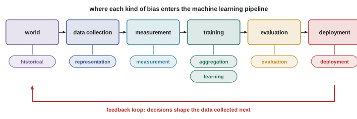
One useful framework, developed by Suresh and Guttag, names seven sources along the machine learning pipeline:

• Historical bias: the world itself reflects past and present inequality, so even perfectly measured data reproduce it.
• Representation bias: some groups are under-represented or missing from the data used to train the model.
• Measurement bias: the features or labels are measured differently, or less accurately, for some groups, or are poor proxies for the quantity of interest.
• Aggregation bias: a single model is used for groups whose relationships between features and outcomes genuinely differ.
• Learning bias: modelling choices, such as the objective or regularization, amplify disparities, for example by optimizing overall accuracy dominated by the majority group.
• Evaluation bias: the benchmark or test set does not represent the population the model will serve, so problems go unseen.
• Deployment bias: the system is used in a way that differs from what it was designed for, or people interact with its outputs inconsistently.

Historical bias

Historical bias exists even when data are measured perfectly. If women were historically excluded from certain roles, a model trained on past hiring decisions learns that men are more likely to be hired; if neighbourhoods were denied investment for decades, property values and credit histories reflect that. A well-known example is a hiring screen trained on ten years of résumés that learned to penalize words associated with women, such as the names of women's colleges, because the historical hires were mostly men. The model accurately reflected the past; the problem was using the past as the definition of a good candidate.

Addressing historical bias usually requires a deliberate choice about the target. Is the goal to predict what decision-makers did in the past, or what outcome a person would achieve if given the opportunity? The second is often what is wanted but is harder to measure, because outcomes are only observed for people who were given the opportunity, a problem called selective labels.

Representation bias

Representation bias occurs when training data under-sample some groups. Face analysis benchmarks once consisted mostly of lighter-skinned faces; the Gender Shades study found commercial gender classifiers had error rates under 1 % for lighter-skinned men but over 30 % for darker-skinned women. Speech data sets over-represent certain accents; medical imaging data come mostly from a few large hospitals; text corpora over-represent some languages and dialects. Models trained on such data learn the majority well and the minority poorly, because the training loss is dominated by the majority. Sampling more data from under-represented groups, data augmentation, and evaluating each group separately are the main remedies, but collecting representative data often requires partnerships and consent processes, not just more scraping.

Measurement bias and proxy labels

Measurement bias arises when the variables used are imperfect proxies, and the imperfection differs by group. Arrest records are a proxy for crime, but arrests depend on where police patrol; healthcare spending is a proxy for health need, but spending depends on access to care. A landmark study by Obermeyer and colleagues found that an algorithm used to allocate care management for millions of US patients predicted future healthcare costs. Because less money was historically spent on Black patients with the same level of illness, the algorithm assigned them lower risk scores; at a given score, Black patients were considerably sicker. Changing the target from cost to direct measures of health need greatly reduced the disparity. The lesson is general: check whether the label measures what you care about equally well for every group.

Features can also be measured differently. Pulse oximeters, which estimate blood oxygen, have been shown to overestimate oxygen levels in patients with darker skin, so models that use oximeter readings inherit that error. Survey data collected only in one language, or images captured with cameras tuned for lighter skin, carry similar problems into the features.

Proxies and fairness through unawareness

Removing a sensitive attribute does not remove its influence. Postal code, first name, school attended, shopping patterns and even typing style can correlate with race, sex or age. A model trained without the sensitive attribute will use these proxies if they help predict a biased label. Worse, removing the attribute makes it harder to detect and correct the problem. Testing whether a model's inputs can predict the sensitive attribute is a simple diagnostic: if a classifier can recover group membership from the features with high accuracy, the information is present.

Aggregation, learning and evaluation bias

Aggregation bias occurs when one model is fitted to groups that differ in meaningful ways. In medicine, the relationship between a biomarker and disease can differ by sex or ancestry; a single model calibrated on the combined data can be wrong for each group. Learning bias arises when the training objective favours the majority: minimizing average loss puts little weight on errors for small groups, and techniques such as aggressive pruning, quantization or differential privacy can degrade minority-group performance more than average performance. Evaluation bias arises when benchmarks do not represent the deployment population, so a model can top a leaderboard while failing for the people it will actually serve. Disaggregated evaluation on representative test data is the safeguard.

Feedback loops

Deployed models change the world that produces their future training data. Predictive policing is the classic example: if patrols are sent where past records show the most incidents, more incidents are recorded there, simply because officers are present to observe them, and the next model sends even more patrols. Recommender systems create similar loops: content that is shown gets clicked, clicks become training data, and popular items become more popular regardless of quality.

import numpy as np
# A feedback loop: patrols go where past records are, and records come from patrols
rng = np.random.default_rng(2)
true_rate = np.array([0.10, 0.10])          # two districts with identical true incident rates
records = np.array([60.0, 40.0])            # historical records start slightly unequal
patrols_total = 100
print("year  patrol_share_A  records_A  records_B  share_of_records_A")
for year in range(1, 11):
    share_a = records[0] ** 2 / (records[0] ** 2 + records[1] ** 2)   # hot spot rule favors the larger count
    patrols = np.array([share_a, 1 - share_a]) * patrols_total
    observed = rng.poisson(patrols * true_rate * 10)                   # incidents are only seen where officers are
    records = records + observed
    if year in (1, 2, 3, 5, 10):
        print(f"{year:4d}  {share_a:14.2f}  {records[0]:9.0f}  {records[1]:9.0f}  {records[0] / records.sum():18.2f}")
print("true incident rates are equal, yet the data say district A has most of the incidents")

year  patrol_share_A  records_A  records_B  share_of_records_A
   1            0.69        123         76                0.62
   2            0.72        198         98                0.67
   3            0.80        272        118                0.70
   5            0.88        439        144                0.75
  10            0.96        920        183                0.83
true incident rates are equal, yet the data say district A has most of the incidents

Both districts in the simulation have exactly the same true incident rate. District A starts with 60 % of historical records, a small difference that might come from chance or past practice. Because the allocation rule concentrates patrols on the district with more records, and incidents are only recorded where officers patrol, A receives 69 % of patrols in year one and 96 % by year ten, and its share of recorded incidents rises from 60 % to 83 %. A model retrained each year on these records would appear increasingly confident that district A is more dangerous, when the data reflect only where people looked. Breaking such loops requires data that do not depend on the model's own decisions, such as random exploration, independent surveys or victim reports, or explicit correction for exposure.

Deployment and human factors

Bias also enters through how predictions are used. Judges, caseworkers and managers may follow a risk score for some people and override it for others, introducing disparities the model itself does not have. Automation bias leads people to defer to model output even when it is wrong; algorithm aversion leads some to ignore good advice. A model designed to support decisions may be used to make them automatically, or applied in a new region with a different population. Monitoring how outputs are used, not only how accurate they are, is part of a fairness review.

Bias in language and generative models

Large language models and image generators learn from web-scale data that contain the full range of human stereotypes. Word embeddings famously encoded analogies such as "man is to computer programmer as woman is to homemaker". Generative models can amplify such associations: asked for images of a chief executive, an early image generator produced mostly men; asked to complete sentences about different religions, a language model associated some with violence far more than others. Lesson 6 covers how to measure and mitigate these representational harms.

Diagnosing bias in a project

A practical diagnosis asks a structured set of questions. Who is in the data, and who is missing compared with the population served? How were labels produced, by whom, and do they measure the intended outcome equally well across groups? Which features might act as proxies for sensitive attributes? Are error rates and outcomes reported by group on representative test data? Could the model's decisions affect its own future training data? How will people use the outputs? Writing the answers down, ideally in a datasheet and model card (Lesson 11), turns vague concern into specific risks with owners.