
STAT-235 · Lesson 4 of 5 · 35 min
Confidence intervals and hypothesis tests
An engineer never sees the whole population. We test twenty concrete cylinders, not the whole pour; eight rebar coupons, not the whole heat of steel; ten asphalt slabs, not the whole highway. Statistical inference is the reasoning that takes us from a sample to a justified statement about the population, with an honest measure of how sure we can be. This chapter covers the two main tools: confidence intervals, which estimate a quantity with a margin of error, and hypothesis tests, which decide whether data provide convincing evidence for a claim.
From sample to population
A population parameter, such as the true mean strength μ, is fixed but unknown. A sample statistic, such as the sample mean \(\bar{x}\), is known but varies from sample to sample. Lesson 3 showed how much: the sample mean has standard deviation \(\sigma/\sqrt{n}\) and is approximately normal. That standard deviation of a statistic is called its standard error. Because σ is usually unknown too, we estimate the standard error with the sample standard deviation s:
Inference needs a sample that represents the population. Random sampling (every unit has a chance of selection) is the foundation; a sample of the cylinders that "looked good", or only from the morning trucks, can be wrong in a way no formula can fix.
Confidence intervals for a mean
A confidence interval gives a range of plausible values for a parameter. For a population mean with σ unknown, it uses Student's t distribution:
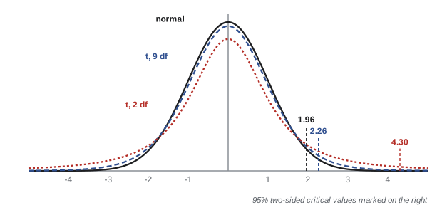
The t distribution looks like the standard normal but has heavier tails, to allow for the extra uncertainty of estimating σ from the sample. It depends on the degrees of freedom n − 1; as n grows it approaches the normal. For 95% confidence, t is 2.776 with 4 degrees of freedom, 2.262 with 9, 2.093 with 19 and approaches 1.96 for large samples.
Worked problem
Mean strength of a pour
The 20 cylinders from Lesson 1 had mean 5430.5 psi and standard deviation 433 psi. Find a 95% confidence interval for the mean strength of the concrete in the pour.
Show solution
- \(SE = 433/\sqrt{20} = 96.8\) psi; \(t_{0.025,19} = 2.093\).
- Margin of error \(= 2.093 \times 96.8 = 203\) psi.
- \[5430 \pm 203 \Rightarrow (5228,\ 5633)\ \text{psi}\]
Answer: We are 95% confident the mean strength of the pour is between about 5230 and 5630 psi
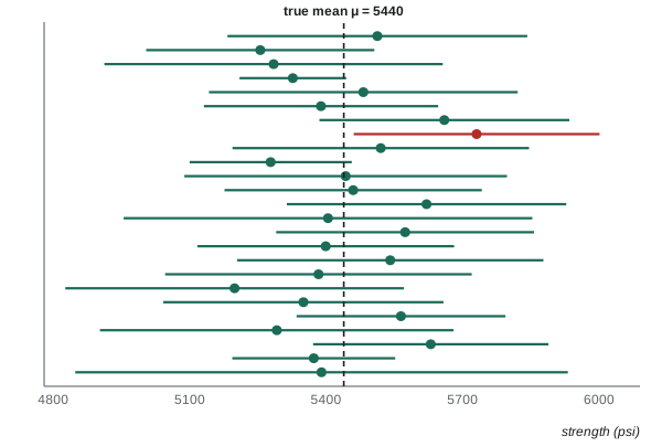
What does "95% confident" mean? The method, used over and over on new samples, produces intervals that contain the true mean 95% of the time. Any one interval either contains μ or does not; we just do not know which. It does not mean 95% of individual cylinders lie in the interval: the interval is about the mean, and it shrinks as n grows, while the spread of individual values does not.
Choosing the sample size
Solving the margin of error for n gives the sample size needed to estimate a mean to within ±E, using a planning value for σ from past data:
Worked problem
How many cylinders?
With σ ≈ 430 psi from past pours, how many cylinders are needed to estimate the mean strength within ±150 psi at 95% confidence?
Show solution
- \(n = (1.96 \times 430 / 150)^2 = 31.6\), rounded up to 32.
Answer: 32 cylinders. Halving the margin to ±75 psi would need four times as many, 127: precision is expensive
Confidence interval for a proportion
For a proportion, such as the fraction of defective items or of homes with a particular feature, with x successes in n trials and \(\hat{p} = x/n\), a large-sample 95% interval is
Worked problem
Lead service lines
A city excavates 400 randomly selected water service connections and finds 52 made of lead. Estimate the proportion of lead service lines city-wide with a 95% confidence interval.
Show solution
- \(\hat{p} = 52/400 = 0.130\); \(SE = \sqrt{0.13 \times 0.87/400} = 0.0168\).
- \(0.130 \pm 1.96(0.0168) = 0.130 \pm 0.033\).
Answer: Between 9.7% and 16.3% of service lines are lead. The replacement budget can be planned on this range rather than a single guess
Hypothesis testing
A hypothesis test asks whether the data provide convincing evidence against a default claim. The procedure is the same for every test:
- State the null hypothesis H₀ (the default, "no effect" or "meets the claim", always an equality such as μ = 400) and the alternative H₁ (what we want evidence for: μ > 400, μ < 400, or μ ≠ 400).
- Choose a significance level α, the risk of wrongly rejecting H₀ you will accept; 0.05 is common.
- Compute a test statistic measuring how far the data are from H₀, in standard errors.
- Find the p-value: the probability, if H₀ were true, of a result at least as extreme as the one observed.
- If p < α, reject H₀: the data are inconsistent with it. Otherwise, fail to reject: the data are consistent with H₀, which is not the same as proving it.
For a mean, the test statistic is
Worked problem
Does the rebar meet its grade?
Reinforcing bar is ordered as ASTM A615 Grade 60, with a specified minimum yield strength of 60 ksi. Eight coupons from a shipment give yield strengths (ksi): 60.75, 62.70, 60.30, 63.15, 61.50, 59.85, 62.25, 63.90. At α = 0.05, is there evidence that the mean yield strength exceeds 60 ksi?
Show solution
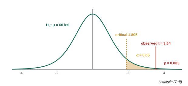
- H₀: μ = 60; H₁: μ > 60 (one-sided).
- \(\bar{x} = 61.80\), \(s = 1.439\), \(SE = 1.439/\sqrt{8} = 0.509\).
- \(t = (61.80 - 60)/0.509 = 3.54\) with 7 degrees of freedom.
- Critical value \(t_{0.05,7} = 1.895\); p-value = 0.005.
Answer: t = 3.54 > 1.895 and p = 0.005 < 0.05: reject H₀. The shipment's mean yield strength convincingly exceeds 60 ksi. (Acceptance in practice also checks individual results, tensile strength, elongation and bend tests against the standard.)
Errors, power and the link to intervals
Two kinds of error are possible. A Type I error rejects a true H₀ (a false alarm) and has probability α. A Type II error fails to reject a false H₀ (a missed effect) and has probability β. The power of a test, 1 − β, is the probability of detecting a real effect of a given size. For a fixed α, power increases with the sample size and with the size of the effect, and decreases with the noise σ.
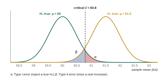
Which error matters more depends on the consequences. Accepting weak steel (failing to detect a strength deficit) is far more serious than rejecting good steel, so acceptance plans are designed to have high power against dangerous deficits. Engineering judgment sets α and the sample size, not convention alone.
Confidence intervals and two-sided tests carry the same information: a two-sided test at α = 0.05 rejects H₀: μ = μ₀ exactly when μ₀ lies outside the 95% confidence interval. Intervals are usually more informative, because they show the size of the effect and its uncertainty, not just a yes or no.
Comparing two means
Independent samples
To compare two groups, such as two mix designs or two suppliers, use the two-sample t test. The Welch version does not assume equal variances and is the safe default:
Its degrees of freedom come from a formula that software computes.
Worked problem
Polymer-modified asphalt
Wheel-tracking tests measure rut depth (mm) on 10 slabs of a conventional asphalt mix and 10 of a polymer-modified mix. Conventional: mean 6.98, s = 0.67. Modified: mean 5.82, s = 0.54. Is there evidence the modified mix ruts less? Estimate the difference.
Show solution
- \(SE = \sqrt{0.67^2/10 + 0.54^2/10} = 0.273\) mm.
- \(t = (6.98 - 5.82)/0.273 = 4.24\) with about 17 degrees of freedom; two-sided p = 0.0005.
- 95% CI for the difference: \(1.16 \pm 2.11(0.273) = (0.58,\ 1.74)\) mm.
Answer: Strong evidence of a difference (p = 0.0005): the modified mix ruts 0.6 to 1.7 mm less in this test. Whether that justifies its extra cost is the engineering question the interval helps answer
Paired samples
When the two measurements come in natural pairs, such as the same specimen measured two ways, or the same site before and after a change, analyze the differences d within each pair with a one-sample t test on the d values. Pairing removes the specimen-to-specimen variation, which can be far larger than the effect of interest.
Worked problem
Do two laboratories agree?
Eight concrete cores are each split, and the halves are tested at two laboratories. Lab 1 (psi): 6110, 5610, 6570, 5830, 5350, 6350, 5730, 6030. Lab 2: 6000, 5540, 6400, 5790, 5220, 6250, 5600, 5980. Is there a systematic difference between the labs?
Show solution
- Differences (Lab 1 − Lab 2): 110, 70, 170, 40, 130, 100, 130, 50. Mean \(\bar{d} = 100\), \(s_d = 44.4\).
- \(t = 100/(44.4/\sqrt{8}) = 6.37\) with 7 degrees of freedom; p = 0.0004.
- For contrast, a (wrong) independent two-sample test on the same numbers gives p = 0.62, because the core-to-core spread of several hundred psi swamps the 100 psi lab difference.
Answer: Lab 1 reads systematically higher, by about 100 psi (p = 0.0004). Using the right test is the difference between detecting the bias and missing it entirely
Running tests in Python
from scipy import stats

rebar = [60.75, 62.70, 60.30, 63.15, 61.50, 59.85, 62.25, 63.90]
r = stats.ttest_1samp(rebar, popmean=60, alternative="greater")
print(f"Rebar: t = {r.statistic:.2f}, p = {r.pvalue:.4f}")

conventional = [6.8, 7.4, 5.9, 8.1, 7.0, 6.5, 7.7, 6.2, 7.3, 6.9]
modified     = [5.6, 6.1, 5.2, 6.8, 5.9, 5.0, 6.4, 5.7, 6.0, 5.5]
r = stats.ttest_ind(conventional, modified, equal_var=False)
print(f"Asphalt (Welch): t = {r.statistic:.2f}, p = {r.pvalue:.4f}")

lab1 = [6110, 5610, 6570, 5830, 5350, 6350, 5730, 6030]
lab2 = [6000, 5540, 6400, 5790, 5220, 6250, 5600, 5980]
r = stats.ttest_rel(lab1, lab2)
print(f"Labs (paired): t = {r.statistic:.2f}, p = {r.pvalue:.4f}")
Output: Rebar: t = 3.54, p = 0.0047; Asphalt (Welch): t = 4.24, p = 0.0005; Labs (paired): t = 6.37, p = 0.0004.
Other tests follow the same logic with different statistics: the chi-square test for counts in categories, the F test and analysis of variance (ANOVA) for comparing more than two means, and non-parametric tests when data are far from normal and samples are small.
Common mistakes
MistakeSaying there is a 95% probability that μ lies in this particular interval.
InsteadThe method captures μ 95% of the time; a given interval either contains it or not.
MistakeUsing z = 1.96 with a small sample and unknown σ.
InsteadUse the t distribution with n − 1 degrees of freedom.
Mistake"Failing to reject H₀ proves H₀ is true."
InsteadIt means the evidence is insufficient; the test may simply lack power.
MistakeReading the p-value as the probability that H₀ is true.
InsteadIt is the probability of data this extreme if H₀ were true.
MistakeAnalyzing paired data as two independent samples.
InsteadTest the within-pair differences; pairing removes unit-to-unit variation.
MistakeEquating statistical significance with practical importance.
InsteadReport the effect size and its confidence interval, and judge it against engineering needs.
Summary and key terms
- The standard error s/√n measures how much a sample mean varies from sample to sample.
- A confidence interval for a mean is x̄ ± t(s/√n); 95% describes the long-run success rate of the method.
- Sample size for margin E: n = (zσ/E)²; halving E quadruples n. Proportions use p̂ ± 1.96√(p̂(1 − p̂)/n).
- Hypothesis tests compute how far data are from H₀ in standard errors; reject H₀ when the p-value is below α.
- Type I error (false alarm, α) and Type II error (missed effect, β) trade off; power 1 − β grows with n and effect size.
- Compare independent groups with the Welch two-sample t test, and paired measurements by testing their differences.
- Parameter
- A fixed, usually unknown, numerical property of a population.
- Statistic
- A number computed from a sample.
- Standard error
- The standard deviation of a statistic, such as s/√n for a mean.
- Confidence interval
- A range, computed from data, that captures the parameter with a stated long-run success rate.
- t distribution
- The distribution used for means when σ is estimated from the sample.
- Degrees of freedom
- The parameter of a t distribution; n − 1 for a one-sample mean.
- Null hypothesis
- The default claim, tested for evidence against it.
- p-value
- The probability, if H₀ is true, of a result at least as extreme as observed.
- Significance level
- The Type I error rate α chosen before testing.
- Type II error
- Failing to reject a false null hypothesis.
- Power
- The probability that a test detects a real effect of a given size.
- Paired test
- A test on within-pair differences for matched measurements.
Practice problems
Work each problem on paper first, then reveal the answer to check.
A sample of 16 has mean 52.0 and s = 4.0. Find a 95% confidence interval for μ (t₀.₀₂₅,₁₅ = 2.131).
Show answer
52.0 ± 2.131 × 1.0 = (49.9, 54.1).
What would happen to the width of that interval with 64 observations and the same s?
Show answer
SE halves (4/8 = 0.5) and t falls to about 2.00, so the interval becomes about ±1.0, less than half as wide.
How many measurements are needed to estimate a mean within ±0.2 mm at 95% if σ ≈ 0.8 mm?
Show answer
(1.96 × 0.8/0.2)² = 61.5 → 62.
In a survey of 250 bridges, 35 have scour-critical foundations. Give a 95% CI for the proportion.
Show answer
p̂ = 0.14; SE = √(0.14 × 0.86/250) = 0.0219; 0.14 ± 0.043 = (0.097, 0.183).
A bolt's nominal length is 50.0 mm. A sample of 25 has mean 50.12 mm and s = 0.30 mm. Test H₀: μ = 50.0 against μ ≠ 50.0 at α = 0.05 (t₀.₀₂₅,₂₄ = 2.064).
Show answer
t = 0.12/0.06 = 2.0 < 2.064: fail to reject. The evidence of a shift is borderline (p ≈ 0.057).
For the previous problem, does the 95% CI contain 50.0?
Show answer
50.12 ± 2.064 × 0.06 = (49.996, 50.244): yes, just, consistent with failing to reject.
A new test procedure would have caught a defect that a factory failed to detect. Which type of error did the factory's test make?
Show answer
Type II: it failed to reject "no defect" when a defect was present.
Name two ways to increase the power of a test without changing α.
Show answer
Increase the sample size; reduce measurement noise (or use a paired design). A larger true effect also raises power.
Two groups: n₁ = n₂ = 12, means 24.5 and 22.1, s₁ = 2.0, s₂ = 2.6. Compute the Welch t statistic.
Show answer
SE = √(4/12 + 6.76/12) = √0.897 = 0.947; t = 2.4/0.947 = 2.53.
Six drivers' reaction times are measured with and without a phone call. Should you use a paired or two-sample test, and why?
Show answer
Paired: the same drivers are measured twice, so testing the differences removes the large driver-to-driver variation.
Lesson quiz · 5 questions
Score 60% or more to complete this lesson.
Create a free account to save your progress, take quizzes and earn a certificate.