Describing data

Engineering decisions rest on measurements, and measurements vary. No two concrete cylinders from the same truck break at exactly the same load; no two bolts from the same machine are exactly the same length; river flow changes every hour. Statistics is the toolkit for making sound decisions when data vary: summarizing what was measured, quantifying uncertainty, and judging whether a difference is real or just noise.

This course covers the statistics every engineer needs. This first chapter is about describing data: types of data and how samples are drawn, the numbers that summarize center and spread, the plots that show shape, and how to spot outliers. The running example is a set of concrete strength tests, the kind of data a site engineer reviews every week.

Populations, samples and data types

A population is the entire set of items or measurements of interest: every cubic yard of concrete placed in a bridge deck, every bolt produced this month. A sample is the part you actually measure, chosen to represent the population. Almost all engineering statistics is about using a sample to learn about a population.

Good conclusions need good samples. A random sample, where every item has an equal chance of selection, avoids systematic bias. Testing only the first bolts off the line each morning, or only the concrete from trucks that arrived on time, could give a misleading picture.

Data come in two broad types:

• Quantitative (numerical): measured values such as strength (psi), length (in) or flow (ft³/s). These may be continuous (any value in a range) or discrete (counts, such as defects per batch).
• Categorical (qualitative): labels such as pass/fail, supplier A/B/C, or failure mode.

Measures of center

The sample mean is the arithmetic average:

The median is the middle value when the data are sorted (the average of the two middle values when n is even). The mode is the most frequent value, mainly useful for categorical data.

The mean uses every value, which makes it efficient but sensitive to extreme values. The median is resistant: one wild value barely moves it. When data are skewed (for example incomes, flood flows, repair times), the mean and median differ, and the median is often the better description of a typical value.

Measures of spread

Two batches can have the same average but very different consistency, and in engineering consistency often matters as much as the average. The standard measures of spread are:

• Range: maximum minus minimum. Simple but depends only on two values.
• Sample variance and standard deviation:

Dividing by \(n - 1\) rather than n corrects for the fact that the deviations are measured from the sample mean rather than the unknown population mean, which makes \(s^2\) an unbiased estimate of the population variance. Calculators and software usually offer both: use the n − 1 version (often labeled s, STDEV.S or ddof=1) for samples.

• Coefficient of variation: \(CV = s/\bar{x}\), the spread relative to the mean, useful for comparing variability between quantities of different size.
• Interquartile range (IQR): the spread of the middle half of the data, \(Q_3 - Q_1\), resistant to outliers.

Quartiles, box plots and outliers

Quartiles divide sorted data into four parts. \(Q_1\) is the median of the lower half, \(Q_3\) the median of the upper half. (Different software uses slightly different rules for interpolating quartiles, so small differences between programs are normal.)

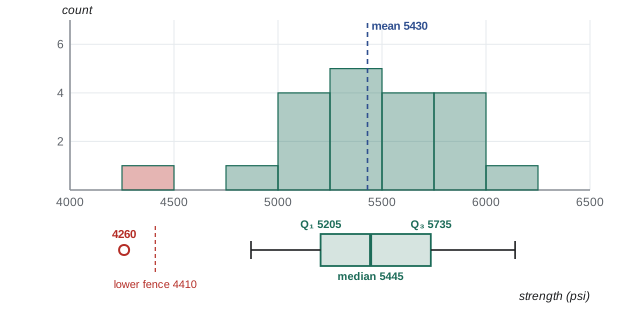
A common rule flags a value as a possible outlier if it lies more than 1.5 IQR below \(Q_1\) or above \(Q_3\). A box plot shows the quartiles as a box, the median as a line inside it, whiskers to the most extreme values within the fences, and outliers as separate points.

This is a crucial engineering point. An outlier is a question, not an error to discard. Removing inconvenient data without cause is both bad statistics and an ethical problem. In concrete practice, ACI 318 sets acceptance criteria for strength tests: every average of three consecutive tests must at least equal the specified strength f′c, and no single test may fall more than 500 psi below f′c (for f′c of 5000 psi or less; above that, more than 10% below). Here f′c = 5000 psi, so 4260 psi (740 psi below) triggers an investigation, often including cores drilled from the structure itself.

Seeing the shape: histograms

A histogram groups the data into bins and draws a bar for the count (or proportion) in each. It shows the shape of the distribution: where it is centered, how spread out it is, whether it is symmetric or skewed, whether it has one peak or several. A rough rule for the number of bins is Sturges' rule, \(k \approx 1 + \log_2 n\), about 5 or 6 bins for 20 values; with more data, more bins reveal more detail.

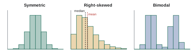
Shape carries engineering information. Many measurement errors and manufactured dimensions are roughly symmetric and bell-shaped. Flood flows, wind speeds, repair times and fatigue lives are typically right-skewed, with occasional very large values, and those extremes usually govern design. A bimodal histogram is a warning that the data mix two populations: two machines, two shifts, two suppliers or two failure modes, which should be separated and analyzed individually.

Standardizing: z-scores

A z-score expresses a value as a number of standard deviations from the mean:

It puts different quantities on a common scale. For roughly bell-shaped data, about 68% of values lie within 1 standard deviation of the mean, 95% within 2, and 99.7% within 3 (the empirical rule, made precise by the normal distribution in Lesson 3). A value with |z| above 3 is unusual.

Relationships between two variables

Often two quantities are measured together: strength and water-cement ratio, deflection and load, fuel use and speed. A scatter plot shows each pair as a point and reveals whether they move together. The sample correlation coefficient r (between −1 and +1) measures the strength of a linear relationship: near ±1 is strong, near 0 is weak. Lesson 5 develops this into regression. For now remember the classic warning: correlation does not by itself show that one variable causes the other, since both may be driven by a third factor.