
ROB-430 · Lesson 9 of 12 · 31 min
Analyzing HRI data
Once a study has been run, its data must be cleaned, described, analyzed and reported honestly. HRI data come in many forms: questionnaire ratings, task times and error counts, robot logs, physiological signals, coded video of behavior and interview transcripts. This lesson focuses on the quantitative core: describing data, comparing conditions with t-tests and their non-parametric alternatives, reporting effect sizes and confidence intervals, measuring agreement between coders with Cohen's kappa, handling multiple comparisons, and understanding why many published findings in psychology and related fields, including HRI, have failed to replicate. The aim is not to make you a statistician, but to let you run and read standard analyses competently and recognize warning signs.
Cleaning and describing data
Analysis starts with checking the data. Are there missing values, and why? Did any participant misunderstand the task, fail attention checks or experience a robot malfunction? Exclusion rules should be decided before seeing the results, ideally in the preregistration, and every exclusion reported. Next, describe the data: means and standard deviations, or medians and interquartile ranges for skewed measures such as task times, and plots that show individual data points, not just bar charts of means. A plot of each participant's scores in both conditions, joined by lines, shows at a glance whether most people moved in the same direction or whether a few extreme cases drive the average.
Questionnaire data need particular care. A single Likert item, such as a five-point agreement rating, is ordinal: the distance between "agree" and "strongly agree" is not necessarily the same as between "neutral" and "agree". Multi-item scales such as the Godspeed subscales or SUS sum or average several items and behave more like interval measures, which is why parametric tests are commonly applied to them. Researchers debate where the line falls; a sensible practice is to analyze validated multi-item scale scores with parametric methods, check results with non-parametric methods when distributions are odd, and avoid treating single items as precise interval measurements. Internal consistency of a scale is commonly reported with Cronbach's alpha, where values above about 0.7 are often considered acceptable, though alpha depends on the number of items and is not proof that a scale measures one thing.
Comparing two conditions
In a within-subjects study comparing two conditions, the paired t-test asks whether the mean of each participant's difference score is different from zero. With \( n \) participants, mean difference \( \bar{d} \) and standard deviation of differences \( s_d \),
The p-value is the probability of a t statistic at least this extreme if the true mean difference were zero. It is not the probability that the hypothesis is true, and a p-value above 0.05 does not show there is no effect. For this reason, results should always include an effect size and a confidence interval. For paired data, \( d_z = \bar{d}/s_d \), and a 95 percent confidence interval for the mean difference is \( \bar{d} \pm t_{0.975, n-1}\, s_d/\sqrt{n} \). For between-subjects designs, Welch's t-test, which does not assume equal variances, is a safe default.
Worked problem
A paired t-test by hand
Ten participants rated perceived safety (1 to 7 scale average) with a robot moving at 0.5 m/s and at 1.0 m/s. Their differences (slow minus fast) have mean 0.62 and standard deviation 0.71. Compute t, \( d_z \) and a 95 percent confidence interval, using \( t_{0.975, 9} = 2.262 \).
Show solution
- Standard error: \( 0.71/\sqrt{10} \approx 0.225 \).
- t: \( 0.62/0.225 \approx 2.76 \) with 9 degrees of freedom, giving \( p \approx 0.02 \).
- Effect size: \( d_z = 0.62/0.71 \approx 0.87 \).
- Interval: \( 0.62 \pm 2.262 \times 0.225 = 0.62 \pm 0.51 \), so 0.11 to 1.13.
Answer: t(9) is about 2.76, p about 0.02, \( d_z \) about 0.87, and the 95 percent interval for the mean difference runs from about 0.11 to 1.13 scale points: the slower speed felt safer, but the size of the effect is uncertain with ten people.
# Paired comparison on synthetic data: t statistic, effect size and a sign-flip permutation p-value
import numpy as np
rng = np.random.default_rng(430)
n = 16
person = rng.normal(4.5, 0.9, n)                       # each participant's typical rating
slow = np.clip(person + 0.35 + rng.normal(0, 0.5, n), 1, 7)
fast = np.clip(person - 0.15 + rng.normal(0, 0.5, n), 1, 7)
d = slow - fast
t = d.mean() / (d.std(ddof=1) / np.sqrt(n))
flips = rng.choice([-1, 1], size=(20000, n))
t_null = (flips * d).mean(axis=1) / ((flips * d).std(axis=1, ddof=1) / np.sqrt(n))
p = np.mean(np.abs(t_null) >= abs(t))
dz = d.mean() / d.std(ddof=1)
boot = np.array([rng.choice(d, n).mean() for _ in range(5000)])
lo, hi = np.percentile(boot, [2.5, 97.5])
print(f"mean difference {d.mean():.2f}, t({n-1}) = {t:.2f}, permutation p = {p:.4f}")
print(f"d_z = {dz:.2f}, bootstrap 95% CI for the mean difference [{lo:.2f}, {hi:.2f}]")
print(f"participants rating slow higher: {np.sum(d > 0)} of {n}")mean difference 0.14, t(15) = 0.84, permutation p = 0.4122 d_z = 0.21, bootstrap 95% CI for the mean difference [-0.19, 0.45] participants rating slow higher: 7 of 16
Look at what happened in this synthetic sample. The simulated true difference between conditions was 0.5 scale points, yet with 16 participants the estimate came out at 0.14, the test was far from significant and the interval included zero. Small samples give noisy estimates in both directions, which is exactly why power analysis (lesson 8) and confidence intervals matter.
When assumptions are doubtful, for example with strongly skewed task times or small samples of ordinal ratings, the Wilcoxon signed-rank test (paired) and the Mann-Whitney U test (independent groups) are common non-parametric alternatives. Permutation tests, like the sign-flip test in the code above, make few assumptions and are easy to explain: if the condition labels did not matter, flipping the sign of each person's difference should produce statistics as extreme as the observed one fairly often. For more than two conditions, analysis of variance (ANOVA) or its repeated-measures version is used, followed by planned comparisons. Increasingly, HRI researchers use linear mixed-effects models, which handle repeated measures, unbalanced data and random effects for both participants and stimuli in one framework.
Agreement between coders: Cohen's kappa
Many HRI measures come from coding video: whether a participant looked at the robot, whether they hesitated, whether a handover succeeded. Because coding involves judgment, two coders should code at least a subset of the data independently, and their agreement should be reported. Raw percentage agreement overstates reliability because coders agree some of the time by chance. Jacob Cohen's kappa corrects for this:
Chance agreement \( p_e \) is computed from each coder's marginal proportions: for each category, multiply the proportion of items coder 1 put in it by the proportion coder 2 put in it, and sum over categories. Richard Landis and Gary Koch suggested in 1977 that kappa values of 0.41 to 0.60 indicate moderate agreement, 0.61 to 0.80 substantial and above 0.80 almost perfect, though they described these bands as arbitrary and kappa depends on category prevalence. For ordered categories, weighted kappa gives partial credit for near misses, and for more than two coders Fleiss' kappa or Krippendorff's alpha are used.
Worked problem
Cohen's kappa by hand
Two coders label 100 video clips as hesitation or no hesitation. Both say hesitation for 20 clips, both say no hesitation for 60, coder 1 says hesitation and coder 2 no for 8, and coder 1 no and coder 2 hesitation for 12. Compute percentage agreement and kappa.
Show solution
- Observed agreement: \( p_o = (20 + 60)/100 = 0.80 \).
- Coder 1 hesitation proportion: \( (20 + 8)/100 = 0.28 \); coder 2: \( (20 + 12)/100 = 0.32 \).
- Chance agreement: \( p_e = 0.28 \times 0.32 + 0.72 \times 0.68 = 0.0896 + 0.4896 = 0.579 \).
- Kappa: \( (0.80 - 0.579)/(1 - 0.579) = 0.221/0.421 \approx 0.52 \).
Answer: Agreement is 80 percent but kappa is only about 0.52, moderate; the coding scheme probably needs clearer definitions of hesitation and coder training.
# Cohen's kappa for two coders on synthetic video codes
import numpy as np
rng = np.random.default_rng(430)
cats = ["look_robot", "look_task", "look_away"]
truth = rng.choice(3, size=200, p=[0.5, 0.35, 0.15])
def coder(acc):
    c = truth.copy(); wrong = rng.random(truth.size) > acc
    c[wrong] = rng.choice(3, size=wrong.sum()); return c
a, b = coder(0.85), coder(0.80)
cm = np.zeros((3, 3), int)
np.add.at(cm, (a, b), 1)
n = cm.sum(); po = np.trace(cm) / n
pe = np.sum(cm.sum(axis=1) * cm.sum(axis=0)) / n**2
kappa = (po - pe) / (1 - pe)
print("confusion matrix (coder A rows, coder B columns):"); print(cm)
print(f"observed agreement {po:.3f}, chance agreement {pe:.3f}, kappa {kappa:.3f}")confusion matrix (coder A rows, coder B columns): [[82 12 8] [11 49 5] [ 5 6 22]] observed agreement 0.765, chance agreement 0.388, kappa 0.616
Many tests, many chances
Each statistical test at the 0.05 level has a 5 percent chance of a false positive when there is no effect. A study that tests 20 independent outcomes has about a 64 percent chance of at least one false positive (\( 1 - 0.95^{20} \)). HRI studies often measure many outcomes: every Godspeed subscale, every NASA-TLX subscale, task time, errors and more. Corrections for multiple comparisons control this. The Bonferroni correction tests each of \( m \) hypotheses at \( \alpha/m \). The Holm procedure is uniformly more powerful: sort the p-values from smallest to largest, compare the \( k \)-th smallest with \( \alpha/(m - k + 1) \), and stop at the first one that fails. Alternatively, designating one primary outcome in advance, with others treated as secondary or exploratory, keeps the main conclusion clean.
Worked problem
Holm correction
A study tests four outcomes and obtains p-values 0.004, 0.030, 0.012 and 0.200. Which are significant at a family-wise 0.05 level using Bonferroni and using Holm?
Show solution
- Bonferroni threshold: \( 0.05/4 = 0.0125 \); significant: 0.004 and 0.012.
- Holm: sort to 0.004, 0.012, 0.030, 0.200.
- Compare 0.004 with \( 0.05/4 = 0.0125 \): pass. Compare 0.012 with \( 0.05/3 \approx 0.0167 \): pass. Compare 0.030 with \( 0.05/2 = 0.025 \): fail, so stop.
Answer: Both methods find the outcomes with p = 0.004 and p = 0.012 significant; here Holm gives the same result, but it can reject more hypotheses when several p-values are moderately small.
The replication crisis
In 2015 the Open Science Collaboration published an attempt to replicate 100 studies from three leading psychology journals. While 97 percent of the original studies had reported statistically significant results, only about 36 percent of the replications did, and replication effect sizes were on average about half the original ones. Similar projects in economics, cancer biology and social science found varying but often disappointing replication rates. HRI borrows methods from psychology and has many of the same risk factors: small samples, many measured outcomes, flexible analysis choices, novel and unreplicated effects, and publication incentives that favor striking positive findings. Researchers in HRI have called for more replication, preregistration and larger samples.
Several practices produce false or inflated findings. P-hacking means trying different analyses, exclusions or outcomes until something crosses p < 0.05. HARKing, hypothesizing after the results are known, presents an exploratory finding as if it had been predicted. The garden of forking paths, a term from Andrew Gelman and Eric Loken, describes how even without deliberate fishing, data-dependent analysis decisions make false positives more likely. Publication bias means that studies with null results stay in file drawers. And small studies suffer from the winner's curse: among small studies, those that happen to reach significance are the ones that overestimated the effect, so published effects are inflated.
# The winner's curse: small studies that reach significance overestimate the true effect
import numpy as np
rng = np.random.default_rng(430)
true_d = 0.3
for n in (15, 40, 150):                                  # per group, two-group design
    est, sig = [], []
    for _ in range(4000):
        a = rng.normal(0, 1, n); b = rng.normal(true_d, 1, n)
        sp = np.sqrt((a.var(ddof=1) + b.var(ddof=1)) / 2)
        d = (b.mean() - a.mean()) / sp
        t = (b.mean() - a.mean()) / (sp * np.sqrt(2 / n))
        est.append(d); sig.append(abs(t) > 1.98)
    est, sig = np.array(est), np.array(sig)
print(f"n = {n:3d}: power {sig.mean():.2f}, mean d among significant results {est[sig].mean():.2f} (true {true_d})")n = 15: power 0.14, mean d among significant results 0.89 (true 0.3) n = 40: power 0.27, mean d among significant results 0.59 (true 0.3) n = 150: power 0.73, mean d among significant results 0.36 (true 0.3)
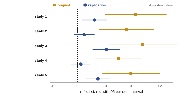
The remedies are well established. Preregister hypotheses, sample sizes and analysis plans. Consider registered reports, in which a journal reviews and accepts the study design before data are collected, so publication does not depend on the result. Compute sample sizes from realistic effect sizes, which are often smaller than published ones. Report all measured outcomes and all conditions. Share data, analysis code and materials so that others can check and reuse them. Report effect sizes with confidence intervals rather than only p-values. Run replications, including of your own key findings, and treat exploratory results as hypotheses for future studies rather than conclusions.
Reporting results
A good results section reports what was planned and what was done, the number of participants analyzed and any excluded, descriptive statistics for every condition, the test used and why, test statistics with degrees of freedom, exact p-values, effect sizes with confidence intervals, and plots that show the data. For example: perceived safety was higher at 0.5 m/s (mean 5.4, SD 0.8) than at 1.0 m/s (mean 4.8, SD 0.9), t(15) = 3.1, p = 0.007, \( d_z \) = 0.78, 95 percent CI for the difference [0.19, 1.01]. Qualitative data from interviews or open-ended responses should be analyzed systematically, for example with thematic analysis, and reported with enough detail that readers can judge the interpretation.
| Situation | Common analysis | Report |
|---|---|---|
| Two conditions, within subjects, scale scores | Paired t-test or Wilcoxon signed-rank | t, df, p, \( d_z \), CI |
| Two independent groups | Welch's t-test or Mann-Whitney U | t, df, p, d, CI |
| Three or more conditions | Repeated-measures ANOVA or mixed-effects model | F, df, p, effect size, planned contrasts |
| Video coding reliability | Cohen's kappa, weighted kappa or Krippendorff's alpha | Kappa and share of data double-coded |
| Scale reliability | Cronbach's alpha or omega | Coefficient for each scale in this sample |
| Many outcomes | Holm or Bonferroni, or one primary outcome | Corrected and uncorrected results |
Common mistakes
MistakeReporting only p-values.
InsteadReport effect sizes and confidence intervals alongside test results.
MistakeInterpreting p > 0.05 as proof of no effect.
InsteadA non-significant result may reflect low power; report the interval and consider equivalence tests.
MistakeReporting percentage agreement for video coding.
InsteadUse Cohen's kappa or a similar chance-corrected statistic.
MistakeTesting many outcomes and highlighting whichever is significant.
InsteadCorrect for multiple comparisons or designate a primary outcome in advance.
MistakeTreating a single small significant study as an established effect.
InsteadExpect inflated effects; look for replication and preregistered confirmation.
Summary and key terms
- Check, clean and describe data before testing, with exclusion rules set in advance.
- Single Likert items are ordinal; validated multi-item scales are commonly analyzed parametrically.
- Paired t-tests compare within-subjects conditions; report \( d_z \) and a confidence interval.
- Non-parametric and permutation tests are alternatives when assumptions are doubtful.
- Cohen's kappa corrects coder agreement for chance.
- Multiple comparisons inflate false positives; Holm and Bonferroni corrections control them.
- The replication crisis showed that small, flexible, unpreregistered studies often fail to replicate.
- Paired t-test
- A test of whether the mean within-person difference differs from zero.
- Effect size
- A measure of the magnitude of an effect, such as Cohen's d.
- Confidence interval
- A range of plausible values for a parameter at a stated confidence level.
- Permutation test
- A test that compares a statistic with its distribution under random relabeling.
- Cohen's kappa
- A chance-corrected measure of agreement between two raters.
- Cronbach's alpha
- A measure of internal consistency of a multi-item scale.
- Holm procedure
- A step-down correction controlling family-wise error across multiple tests.
- P-hacking
- Trying analyses until a significant result appears.
- HARKing
- Hypothesizing after the results are known.
- Registered report
- A publication format in which the design is peer reviewed and accepted before data collection.
Practice problems
Work each problem on paper first, then reveal the answer to check.
Mean difference 1.0, SD of differences 2.0, n = 16: t?
Show answer
\( 1.0/(2.0/4) = 2.0 \).
For the previous question, what is \( d_z \)?
Show answer
0.5.
\( p_o = 0.9 \), \( p_e = 0.5 \): kappa?
Show answer
0.8.
Chance of at least one false positive in 10 independent tests at 0.05?
Show answer
\( 1 - 0.95^{10} \approx 0.40 \).
Bonferroni threshold for 5 tests at 0.05?
Show answer
0.01.
What share of replications in the 2015 Open Science Collaboration project were significant?
Show answer
About 36 percent.
Define HARKing.
Show answer
Presenting a hypothesis formed after seeing the data as if it had been predicted.
Why do small significant studies overestimate effects?
Show answer
Only the samples that happened to overestimate cross the significance threshold.
Name a non-parametric alternative to the paired t-test.
Show answer
The Wilcoxon signed-rank test, or a sign-flip permutation test.
What should be reported with each test?
Show answer
Statistic, degrees of freedom, exact p, effect size and confidence interval.
Lesson quiz · 5 questions
Score 60% or more to complete this lesson.
Create a free account to save your progress, take quizzes and earn a certificate.