
ROB-410 · Lesson 7 of 12 · 29 min
Simulation for robot learning
Lesson 5 showed that a modern on-policy algorithm can consume a hundred million environment steps before a locomotion policy works well. No physical robot can supply that. Simulation can: a single workstation with a modern graphics processor can step thousands of simulated robots in parallel, faster than real time, with no wear, no resets by people and no risk of damage. Simulation has therefore become the main source of experience for reinforcement learning in robotics, and a growing source of synthetic data for imitation and perception. The catch is that a policy trained in simulation must still work on a real robot. This lesson covers how robot-learning simulators work, how to make policies robust to the differences between simulation and reality, and how curricula and parallelism make training practical. ROB-360 covered simulation fundamentals, physics engines, models and the basics of sim-to-real transfer; here we focus on what is specific to learning.
What a learning simulator needs
A simulator for robot learning must do four things well. It must be fast, because learning needs enormous numbers of steps; throughput, measured in total environment steps per second across all parallel copies, matters more than the speed of any single copy. It must be physically plausible for the contacts that matter to the task, such as feet on terrain or fingertips on objects. It must produce the observations the real robot will see, which may include joint encoders, force sensors, depth images or color images. And it must be controllable from code, so that every parameter, from object masses to lighting, can be changed at each reset.
At the time of writing (October 2026), several open-source and commercial platforms meet these needs to different degrees. GPU-based simulators such as NVIDIA's Isaac Sim and its Isaac Lab learning framework run thousands of environments on one graphics card. MuJoCo, open-sourced in 2022 and now with GPU-accelerated variants, is widely used for contact-rich control research. PyBullet, Gazebo and Webots remain common for smaller experiments and ROS-based workflows. Libraries change quickly; the concepts in this lesson apply to all of them.
| Requirement | Why it matters for learning | How simulators provide it |
|---|---|---|
| Throughput | RL needs millions to billions of steps | Thousands of environments stepped in parallel on a GPU |
| Contact fidelity | Policies exploit contact behavior | Careful contact models, small time steps, tuned friction |
| Sensor rendering | Vision policies need realistic images | Rasterized or ray-traced cameras, depth noise models |
| Randomization hooks | Robustness needs variation at every reset | Programmatic access to masses, friction, textures, lighting |
| Determinism and seeding | Debugging and fair comparisons | Fixed seeds and reproducible stepping |
Worked problem
Throughput and wall-clock time
A locomotion policy needs about \( 2 \times 10^8 \) environment steps. A GPU simulator runs 4,096 environments at an aggregate 150,000 steps per second including policy inference and learning updates. How long does training take? How long would it take at real-time speed on one physical robot at 50 Hz?
Show solution
- Simulation: \( 2 \times 10^8 / 1.5 \times 10^5 \approx 1333 \) s, about 22 minutes.
- Physical robot: \( 2 \times 10^8 / 50 = 4 \times 10^6 \) s.
- That is about 46 days of continuous operation, ignoring resets, charging and repairs.
Answer: About 22 minutes in simulation against roughly 46 days of non-stop real operation, which is why large-scale RL is done in simulation.
The reality gap
A policy trained in simulation inherits every assumption the simulator makes. Real motors have backlash, friction that changes with temperature, current limits and communication delays. Real contacts are softer or stiffer than modeled, and friction coefficients vary from surface to surface. Real cameras have noise, motion blur, lens distortion and changing lighting. Real objects have masses and inertias that differ from their nominal values. The difference between simulated and real behavior is called the reality gap, or the sim-to-real gap.
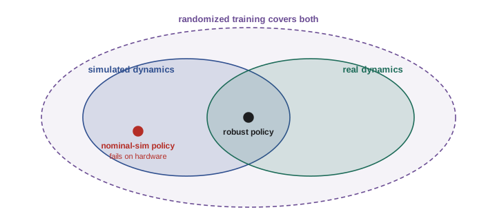
Learning makes the gap more dangerous than it is for hand-designed controllers. An optimizer searching over millions of trials will find and rely on any quirk of the simulator that helps it score: a contact model that allows a foot to slide without resistance, a gripper that never slips, a joint that responds instantly. Such a policy can look excellent in simulation and fail immediately on hardware. The tools below aim to train policies that do not depend on those quirks.
Domain randomization
Domain randomization trains the policy across many variations of the simulator, so that the real world looks like just one more variation. At each episode reset, physical parameters are drawn from ranges: masses, friction coefficients, motor strength, joint damping, sensor noise, control latency, and for vision policies also textures, colors, lighting, camera pose and distracting objects. A policy that succeeds across the whole range cannot depend on any single value, so it is more likely to work at the real values, which are never known exactly.
Choosing ranges is a balancing act. Ranges that are too narrow may not include reality. Ranges that are too wide make the task harder than necessary and can produce timid, overly conservative policies that perform poorly everywhere. A good starting point is to measure the real parameters as well as possible, as ROB-360's system identification lesson described, and then randomize around those measurements with ranges that reflect the remaining uncertainty, plus some margin. Randomizing latency and action delays is particularly important for dynamic tasks, because many sim-to-real failures come from timing rather than from physics.
# Why randomization helps: tune a push force on a nominal sim vs a randomized sim
import numpy as np
rng = np.random.default_rng(3)
def slides_to_target(force, mu, m=1.0, push_time=0.3, g=9.81, target=(0.45, 0.55)):
    # Push a block with constant force for push_time, then let friction stop it.
    a_push = force / m - mu * g
    if a_push <= 0:
        return False
    v = a_push * push_time
    d = 0.5 * a_push * push_time**2 + v**2 / (2 * mu * g)
    return target[0] <= d <= target[1]
forces = np.linspace(3, 12, 181)
mu_nominal = 0.30
best_nominal = max(forces, key=lambda f: slides_to_target(f, mu_nominal) - abs(f - 6.0) * 1e-6)
mus_train = rng.uniform(0.22, 0.40, 400)            # randomized friction in training
rate = [np.mean([slides_to_target(f, mu) for mu in mus_train]) for f in forces]
best_random = forces[int(np.argmax(rate))]
mus_real = rng.normal(0.33, 0.03, 2000)             # "reality": unknown, slightly different
for name, f in (("nominal-tuned", best_nominal), ("randomized-tuned", best_random)):
    real = np.mean([slides_to_target(f, mu) for mu in mus_real])
print(f"{name:17s} force {f:5.2f} N -> real success {real:.1%}")nominal-tuned force 7.10 N -> real success 14.1% randomized-tuned force 7.90 N -> real success 47.9%
Worked problem
Setting a randomization range
System identification estimates a gripper's fingertip friction coefficient as 0.55 with a standard deviation of 0.05 across test objects, and the real robot's control latency as 18 ms to 30 ms. Propose training ranges.
Show solution
- Friction: cover about three standard deviations plus margin, for example 0.35 to 0.75.
- Latency: cover the measured range with margin, for example 10 ms to 40 ms, sampled at each reset.
- Check that the policy can still succeed at the extremes; if it cannot, the range may be too wide or the task needs a different strategy.
- After the first real trials, narrow or shift the ranges if failures cluster at particular values.
Answer: Friction about 0.35 to 0.75 and latency about 10 ms to 40 ms, refined after real-world testing.
Beyond uniform randomization
Several refinements improve on picking fixed ranges by hand. Automatic domain randomization starts with narrow ranges and widens each one whenever the policy performs well at its edges, so the difficulty grows with the policy's ability. Adaptive or system-identification-in-the-loop approaches use real-world data to adjust the simulator's parameter distribution so that simulated trajectories match real ones more closely. Privileged-information training, sometimes called teacher-student training, first trains a teacher policy that can see true simulator parameters such as friction and terrain height, then trains a student policy that sees only the real robot's sensors to imitate the teacher. The student learns to infer hidden parameters from its recent history of observations and actions, which has proved very effective for legged locomotion over rough terrain.
Curricula
Many tasks are too hard to learn from scratch: a quadruped that has not learned to stand will never discover how to climb stairs. A curriculum orders training from easy to hard. It can change the environment, for example starting on flat ground and gradually raising terrain roughness; change the goal, for example starting with targets near the hand and moving them farther away; or change the reward, for example starting with dense shaping and fading it out. Automatic curricula promote each parallel environment to harder settings when its policy succeeds often enough and demote it when it fails, so that every environment trains near the edge of the policy's ability.
Worked problem
An automatic terrain curriculum
Terrain difficulty levels run from 0 (flat) to 9 (steep steps). An environment moves up one level when the robot walks more than 80 % of the commanded distance in an episode and down one level when it walks less than 40 %. A robot at level 4 achieves 85 %, 90 %, 35 % and 82 % in four successive episodes. What levels does it visit?
Show solution
- Episode 1 at level 4: 85 % > 80 %, so move to level 5.
- Episode 2 at level 5: 90 %, move to level 6.
- Episode 3 at level 6: 35 % < 40 %, move down to level 5.
- Episode 4 at level 5: 82 %, move to level 6.
Answer: Levels 4, 5, 6, 5, then 6. The environment settles near the hardest terrain the policy can handle.
Parallel environments in practice
GPU simulation changes how training code is organized. Instead of one environment at a time, the code works with tensors holding the states of all environments at once; every operation, from computing rewards to resetting environments that have finished, is vectorized. Environments finish at different times, so resets are handled per environment within the batch. Observation normalization statistics, curricula and randomization are maintained for the whole batch. Large batches of experience suit on-policy algorithms such as PPO, while off-policy methods benefit less because the bottleneck shifts from collecting data to training on it.
# Isaac Lab / Gymnasium style vectorized loop (listing only, not run here)
import torch
obs, info = env.reset()                         # obs: tensor [num_envs, obs_dim]
for it in range(num_iterations):
    for t in range(steps_per_update):           # collect a rollout from all envs at once
        with torch.no_grad():
            dist = policy(normalizer(obs))
            act = dist.sample()
        next_obs, rew, terminated, truncated, info = env.step(act)
        buffer.add(obs, act, rew, terminated, truncated, dist.log_prob(act))
        obs = next_obs                          # finished envs are reset inside env.step
    ppo.update(buffer)                          # several epochs of mini-batch updates
    curriculum.update(info["episode_progress"])
Validating transfer
Transfer should be tested in stages rather than in one leap. First, evaluate the trained policy in simulation under parameter values outside its training ranges to see how quickly performance degrades. Second, run it in a second simulator or with a more detailed model, which catches dependence on one engine's quirks. Third, test on the real robot at reduced speed and in a protected setting, logging everything. Fourth, compare real and simulated trajectories for the same commands, which often reveals a specific mismatch, such as a slower actuator response or higher friction, that can be fixed by improving the model or widening randomization. Finally, measure real-world success rates with confidence intervals, as lesson 12 describes, before increasing autonomy. ROB-360 covered metrics for quantifying the reality gap, such as comparing distributions of key trajectory features between simulation and reality.
| Transfer failure | Typical cause | Remedy |
|---|---|---|
| Jittery, oscillating motion on hardware | Unmodeled latency or motor dynamics | Randomize latency, add actuator models, penalize action changes |
| Slipping or dropping objects | Friction or contact stiffness too optimistic | Randomize friction lower, model fingertip compliance |
| Vision policy fails under new lighting | Too little visual variation | Randomize textures, lighting and camera pose; use pretrained encoders |
| Works in one lab, fails in another | Overfitting to environment details | Randomize backgrounds and layouts; test in several places |
| Gradual degradation over hours | Motor heating, wear, battery voltage | Randomize motor strength; monitor and recalibrate |
Common mistakes
MistakeTraining on a single nominal simulator configuration.
InsteadRandomize physical, sensor and timing parameters around measured values.
MistakeRandomizing everything as widely as possible.
InsteadExcessive ranges produce timid policies; base ranges on measurements and widen only as needed.
MistakeIgnoring latency in simulation.
InsteadModel and randomize control and sensing delays, especially for dynamic tasks.
MistakeGoing straight from simulation to full-speed hardware.
InsteadTest outside training ranges, in a second simulator, then on hardware at reduced speed.
MistakeAssuming high simulated success predicts real success.
InsteadMeasure real success with enough trials and compare real and simulated trajectories.
Summary and key terms
- Simulation provides the vast experience RL needs, with GPU simulators stepping thousands of environments in parallel.
- Learning simulators need throughput, contact fidelity, sensor rendering and programmatic randomization.
- The reality gap is the mismatch between simulated and real behavior, and optimizers exploit simulator quirks.
- Domain randomization trains across parameter ranges so that reality looks like another variation.
- Automatic randomization, adaptive simulation and teacher-student training refine basic randomization.
- Curricula order training from easy to hard, often automatically per environment.
- Transfer should be validated in stages, with real success rates measured before increasing autonomy.
- Reality gap
- The difference between a simulator's behavior and the real world's.
- Sim-to-real transfer
- Deploying a policy trained in simulation on a physical robot.
- Domain randomization
- Varying simulator parameters during training so the policy becomes robust to them.
- Automatic domain randomization
- Widening randomization ranges as the policy improves.
- Privileged information
- Simulator quantities, such as true friction, unavailable to the real robot.
- Teacher-student training
- Training a privileged teacher with RL, then a sensor-only student to imitate it.
- Curriculum
- An ordering of training tasks or conditions from easy to hard.
- Throughput
- Total environment steps per second across all parallel simulations.
- Vectorized environment
- An environment that steps many copies in parallel as a batch.
- System identification
- Estimating physical parameters of a real system from measured data.
Practice problems
Work each problem on paper first, then reveal the answer to check.
Why does throughput matter more than single-environment speed?
Show answer
Learning needs total steps; parallel copies multiply total steps per second.
Give two parameters to randomize for a grasping policy.
Show answer
Object mass, friction, gripper strength, latency, object pose or sensor noise.
Why do optimizers make the reality gap worse?
Show answer
They find and rely on simulator quirks that do not exist in reality.
What is the risk of very wide randomization ranges?
Show answer
Timid, conservative policies that perform poorly everywhere.
What does the student see in teacher-student training?
Show answer
Only the real robot's sensors and its recent history.
A curriculum promotes at 80 % and demotes at 40 %. A result of 60 % does what?
Show answer
Nothing; the environment stays at its level.
How long is \( 10^8 \) steps at 50 Hz in real time?
Show answer
\( 2 \times 10^6 \) s, about 23 days.
Why test a policy in a second simulator?
Show answer
To catch dependence on one engine's quirks.
Name one cause of jittery motion after transfer.
Show answer
Unmodeled latency or motor dynamics.
Which algorithm type benefits most from huge parallel batches?
Show answer
On-policy methods such as PPO.
Lesson quiz · 5 questions
Score 60% or more to complete this lesson.
Create a free account to save your progress, take quizzes and earn a certificate.