
ROB-410 · Lesson 5 of 12 · 31 min
Reinforcement learning II: policy gradients and actor-critic methods
Value-based methods learn how good each action is and then act greedily. For robots with continuous actions, such as joint velocities or end-effector displacements, that greedy step is awkward, because finding the best action means solving an optimization problem at every control step. Policy-gradient methods take a different route: they parameterize the policy directly, for example as a neural network that outputs a distribution over actions, and adjust its parameters in the direction that increases expected return. Actor-critic methods combine the two ideas, using a learned value function to make the policy updates less noisy. Most reinforcement learning for continuous robot control today, including legged locomotion and dexterous manipulation trained in simulation, uses an actor-critic algorithm.
Parameterized stochastic policies
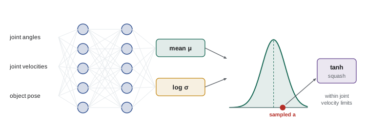
A policy-gradient method represents the policy as \( \pi_\theta(a \mid s) \), a probability distribution over actions whose shape depends on parameters \( \theta \). For continuous actions, the most common choice is a Gaussian: a neural network takes the observation and outputs a mean action \( \mu_\theta(s) \), and a separate parameter or network output gives the standard deviation \( \sigma \). During training, actions are sampled from \( \mathcal{N}(\mu_\theta(s), \sigma^2) \), which provides exploration automatically. At deployment, the robot usually executes the mean action, which is smoother and more repeatable.
Robot actions have limits: joint velocities, torques and workspace boundaries. A common technique is to pass the sampled Gaussian action through a squashing function such as tanh and then scale it to the allowed range, so the policy can never command values outside the limits. Lower-level controllers and safety monitors should still enforce limits independently.
The policy-gradient theorem and REINFORCE
The objective is the expected return \( J(\theta) = \mathbb{E}_{\tau \sim \pi_\theta}[G_0] \), averaged over trajectories \( \tau \) generated by the policy. The policy-gradient theorem gives a way to estimate its gradient from sampled trajectories, without differentiating through the environment's dynamics:
The term \( \nabla_\theta \log \pi_\theta(a_t \mid s_t) \) points in the direction that makes action \( a_t \) more likely in state \( s_t \). It is multiplied by how good the outcome was, \( G_t \), minus a baseline \( b(s_t) \). Actions followed by better-than-baseline returns become more likely; actions followed by worse returns become less likely. The baseline does not change the expected gradient, but a good baseline, usually an estimate of \( V(s_t) \), dramatically reduces variance. The algorithm that applies this estimate directly to complete episodes is called REINFORCE.
REINFORCE is simple and unbiased but very noisy. A single episode's return depends on every random action and every random event, so many episodes are needed per useful update. It is also on-policy: each gradient estimate must come from trajectories generated by the current policy, so old data cannot be reused after the policy changes. Both properties make plain REINFORCE impractical on physical robots, but understanding it is the key to every algorithm that follows.
Worked problem
The log-likelihood gradient for a Gaussian
A one-dimensional Gaussian policy has mean \( \mu \) and fixed standard deviation \( \sigma = 0.5 \). It samples \( a = 2.3 \) when \( \mu = 2.0 \), and the advantage of that action is \( +1.2 \). Compute the policy-gradient contribution for \( \mu \).
Show solution
- For a Gaussian, \( \partial \log \pi / \partial \mu = (a - \mu)/\sigma^2 \).
- \( (2.3 - 2.0) / 0.25 = 1.2 \).
- Multiply by the advantage: \( 1.2 \times 1.2 = 1.44 \).
- A gradient-ascent step with learning rate 0.01 raises \( \mu \) by about 0.0144, toward the better action.
Answer: The contribution is 1.44, which moves the mean toward 2.3, the action that turned out better than average.
# REINFORCE with a baseline on a one-step toy problem: find the action near 3.0
import numpy as np
rng = np.random.default_rng(1)
def reward(a):                       # best action is a = 3.0
    return -(a - 3.0) ** 2
for use_baseline in (False, True):
    mu, sigma, lr, baseline = 0.0, 1.0, 0.02, 0.0
    for it in range(400):
        a = rng.normal(mu, sigma, size=16)          # a batch of 16 one-step episodes
        R = reward(a)
        adv = R - (baseline if use_baseline else 0.0)
        grad = np.mean((a - mu) / sigma**2 * adv)    # d log pi / d mu times advantage
        mu += lr * grad
        baseline = 0.9 * baseline + 0.1 * R.mean()   # running average of returns
    print(f"baseline={use_baseline}: final mu = {mu:.3f}")
# Spread of single-batch gradient estimates at mu = 0, with and without baseline
grads = {False: [], True: []}
for _ in range(2000):
    a = rng.normal(0.0, 1.0, size=16); R = reward(a)
    for b in (False, True):
        adv = R - (R.mean() if b else 0.0)
        grads[b].append(np.mean(a * adv))
for b in (False, True):
print(f"baseline={b}: mean grad {np.mean(grads[b]):5.2f}, std {np.std(grads[b]):5.2f}")baseline=False: final mu = 2.902 baseline=True: final mu = 2.864 baseline=False: mean grad 6.04, std 3.66 baseline=True: mean grad 5.59, std 2.16
Actor-critic methods
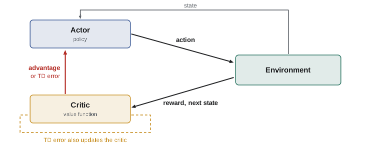
Actor-critic methods replace the Monte Carlo return in REINFORCE with an estimate from a learned value function, the critic. The policy is the actor. The critic, trained by TD learning as in lesson 4, provides an advantage estimate for each step, such as the TD error \( \delta_t = r_{t+1} + \gamma V_\phi(s_{t+1}) - V_\phi(s_t) \), which is an unbiased estimate of the advantage when the critic is accurate. The actor then follows \( \nabla_\theta \log \pi_\theta(a_t \mid s_t)\, \hat{A}_t \). Because the advantage now depends on one or a few steps rather than a whole episode, variance falls sharply, at the cost of some bias from critic errors.
Generalized advantage estimation, or GAE, interpolates between the low-variance one-step TD error and the low-bias Monte Carlo return, using an exponentially weighted sum of TD errors with a parameter \( \lambda \) between 0 and 1:
With \( \lambda = 0 \), GAE is the one-step TD error. With \( \lambda = 1 \), it is the Monte Carlo return minus the value baseline. Values around 0.95 are common in robot locomotion and manipulation training.
Proximal policy optimization
Large policy updates are dangerous: a single bad step can collapse a policy that took hours to train, and on-policy methods cannot easily recover because their new data comes from the broken policy. Trust-region methods limit how far each update can move the policy. Proximal policy optimization, or PPO, achieves this with a simple clipped objective that has become the workhorse of simulated robot learning. Let \( \rho_t(\theta) = \pi_\theta(a_t \mid s_t) / \pi_{\theta_{\text{old}}}(a_t \mid s_t) \) be the ratio of new to old action probabilities. PPO maximizes:
With \( \epsilon \) typically 0.2, the clipping removes any incentive to change an action's probability by more than about 20 % in a single round of updates. PPO collects a batch of experience with the current policy, runs several epochs of mini-batch gradient ascent on this objective, then discards the batch and collects a new one. It is robust to hyperparameters, scales well to thousands of parallel simulated environments and is the default choice in many robot learning frameworks.
Worked problem
Evaluating the PPO clip
For one sample, the old policy gave the action probability density 0.40 and the new policy gives 0.56. The advantage is +2.0. With \( \epsilon = 0.2 \), what is the clipped objective? What if the advantage were −2.0?
Show solution
- Ratio: \( \rho = 0.56/0.40 = 1.4 \).
- Clipped ratio: \( \operatorname{clip}(1.4, 0.8, 1.2) = 1.2 \).
- Positive advantage: \( \min(1.4 \times 2, 1.2 \times 2) = \min(2.8, 2.4) = 2.4 \). The objective stops rewarding further increases.
- Negative advantage: \( \min(1.4 \times -2, 1.2 \times -2) = \min(-2.8, -2.4) = -2.8 \). The unclipped term is kept, so the update is pushed to undo the harmful increase.
Answer: 2.4 for the positive advantage and −2.8 for the negative one. Clipping limits gains from moving too far but never hides losses.
# PPO clipped surrogate for a handful of samples
import numpy as np
ratio = np.array([0.7, 0.9, 1.0, 1.15, 1.4, 1.6])
adv   = np.array([1.0, -1.0, 0.5, 2.0, 2.0, -1.5])
eps = 0.2
unclipped = ratio * adv
clipped = np.clip(ratio, 1 - eps, 1 + eps) * adv
obj = np.minimum(unclipped, clipped)
for r, A, u, c, o in zip(ratio, adv, unclipped, clipped, obj):
    print(f"ratio {r:4.2f}  A {A:5.1f}  unclipped {u:6.2f}  clipped {c:6.2f}  used {o:6.2f}")
print("mean objective:", round(obj.mean(), 3))ratio 0.70 A 1.0 unclipped 0.70 clipped 0.80 used 0.70 ratio 0.90 A -1.0 unclipped -0.90 clipped -0.90 used -0.90 ratio 1.00 A 0.5 unclipped 0.50 clipped 0.50 used 0.50 ratio 1.15 A 2.0 unclipped 2.30 clipped 2.30 used 2.30 ratio 1.40 A 2.0 unclipped 2.80 clipped 2.40 used 2.40 ratio 1.60 A -1.5 unclipped -2.40 clipped -1.80 used -2.40 mean objective: 0.433
Off-policy actor-critic: DDPG, TD3 and SAC
PPO is on-policy, so it needs fresh data for every update. That is fine in a fast simulator but expensive on a real robot. Off-policy actor-critic methods learn a Q-function critic from a replay buffer, like DQN, and train the actor to choose actions that the critic rates highly. Deep deterministic policy gradient, or DDPG, uses a deterministic actor and adds exploration noise. Twin delayed DDPG, or TD3, reduces overestimation by learning two critics and using the smaller of their estimates, and updates the actor less often than the critics. Soft actor-critic, or SAC, uses a stochastic actor and adds an entropy bonus to the objective, rewarding the policy for staying as random as possible while still achieving high return:
The entropy term \( \mathcal{H} \) encourages exploration and makes the policy more robust to small disturbances, and the temperature \( \alpha \) can be tuned automatically to hit a target entropy. Because SAC reuses data, it has been used to learn skills on physical robots, such as walking on a small legged robot or simple manipulation, in hours rather than days of real interaction. On-policy PPO with massive simulation and off-policy SAC with careful real-world data use are the two most common patterns in practice.
| Algorithm | On or off policy | Policy type | Strengths | Typical robot use |
|---|---|---|---|---|
| REINFORCE | On | Stochastic | Simple, unbiased | Teaching, tiny problems |
| PPO | On | Stochastic | Stable, scales to many parallel environments | Locomotion and dexterity in simulation |
| DDPG | Off | Deterministic | Reuses data | Early continuous control work |
| TD3 | Off | Deterministic | Less overestimation than DDPG | Continuous control benchmarks, real arms |
| SAC | Off | Stochastic with entropy bonus | Data efficient, robust exploration | Learning on real hardware, fine-tuning |
Practical details that decide success
Published algorithms are only part of the story. In robot RL, results often depend more on engineering choices than on the algorithm's name. Observations should be normalized, typically by running estimates of their mean and standard deviation, so that joint angles in radians and forces in newtons are on similar scales. Rewards may need scaling so that value targets stay in a reasonable range. The action space should be chosen so that useful behavior is easy to express, which usually means relative position or velocity targets sent to a stiff, well-tuned controller rather than raw torques. Policies trained at one control frequency may behave badly at another, so the deployment rate should match training.
Training curves are noisy, and different random seeds of the same algorithm can give very different results. Report the mean and spread over several seeds, typically five or more, rather than the best run. Watch not only the return but also secondary signals: policy entropy, which should decline gradually; critic loss; the size of each policy update; and simple behavior metrics such as joint-limit violations and action smoothness. Sudden collapses usually point to learning rates that are too high, too few samples per update, or value targets that have grown too large.
Worked problem
How many samples does PPO see?
A PPO run uses 4,096 parallel simulated environments, each collecting 24 steps per update, with 5 epochs of 4 mini-batches per update. Training runs for 1,500 updates. How many environment steps are collected, and how many gradient steps are taken? At 50 Hz, how much simulated experience is this?
Show solution
- Steps per update: \( 4096 \times 24 = 98\,304 \).
- Total steps: \( 98\,304 \times 1500 \approx 1.47 \times 10^8 \).
- Gradient steps: \( 1500 \times 5 \times 4 = 30\,000 \).
- Simulated time: \( 1.47 \times 10^8 / 50 \approx 2.9 \times 10^6 \) s, about 34 days.
Answer: About 147 million steps, roughly 34 days of experience at 50 Hz, gathered in hours of wall-clock time. Collecting this on a real robot would be impossible, which is why on-policy methods rely on simulation.
Common mistakes
MistakeRunning plain REINFORCE on a real robot.
InsteadUse a baseline at minimum, and prefer actor-critic methods; on hardware prefer off-policy methods that reuse data.
MistakeLetting the policy output unbounded actions.
InsteadSquash and scale actions to joint and workspace limits, and keep independent safety limits below the policy.
MistakeReporting the best of several random seeds.
InsteadReport mean and spread over at least five seeds.
MistakeChanging the control frequency at deployment.
InsteadDeploy at the frequency used in training, or train with randomized control rates.
MistakeIgnoring observation normalization.
InsteadNormalize inputs with running statistics so features on different scales do not dominate.
Summary and key terms
- Policy-gradient methods parameterize a stochastic policy and follow the gradient of expected return.
- The policy-gradient theorem weights \( \nabla \log \pi \) by returns minus a baseline; the baseline reduces variance without adding bias.
- Actor-critic methods use a learned critic to estimate advantages, trading a little bias for much lower variance; GAE blends the two.
- PPO clips the probability ratio to keep updates small and is the default for large-scale simulated training.
- Off-policy actor-critics such as TD3 and SAC learn from replay buffers and are more data-efficient on real robots.
- SAC adds an entropy bonus that encourages exploration and robustness.
- Normalization, action-space design, seeds and monitoring often matter more than the choice of algorithm.
- Policy gradient
- The gradient of expected return with respect to policy parameters.
- REINFORCE
- A Monte Carlo policy-gradient algorithm that weights log-probability gradients by returns.
- Baseline
- A value subtracted from returns in policy gradients to reduce variance without bias.
- Actor-critic
- A method that trains a policy (actor) using advantage estimates from a learned value function (critic).
- Generalized advantage estimation
- An exponentially weighted sum of TD errors controlled by \( \lambda \).
- PPO
- Proximal policy optimization, which clips the probability ratio to limit policy changes.
- Probability ratio
- The new policy's action probability divided by the old policy's.
- TD3
- An off-policy deterministic actor-critic with twin critics and delayed actor updates.
- SAC
- Soft actor-critic, an off-policy stochastic actor-critic with an entropy bonus.
- Entropy bonus
- A reward term that favors more random policies to encourage exploration.
Practice problems
Work each problem on paper first, then reveal the answer to check.
What does \( \nabla_\theta \log \pi_\theta(a \mid s) \) point toward?
Show answer
Parameter changes that make action \( a \) more likely in state \( s \).
Why does a baseline not bias the policy gradient?
Show answer
Its expected contribution is zero because the probabilities of all actions sum to one.
Gaussian policy: \( \mu = 1 \), \( \sigma = 1 \), sampled \( a = 0.5 \), advantage −2. Gradient for \( \mu \)?
Show answer
\( (0.5 - 1)/1 \times (-2) = 1 \), so \( \mu \) moves up, away from the bad action.
What does GAE reduce to when \( \lambda = 0 \)?
Show answer
The one-step TD error.
PPO ratio 0.7, advantage −1, \( \epsilon = 0.2 \). Objective?
Show answer
\( \min(-0.7, -0.8) = -0.8 \).
Why is PPO suited to simulation but costly on real robots?
Show answer
It is on-policy and needs fresh data every update.
How does TD3 reduce overestimation?
Show answer
It uses the minimum of two critics' estimates.
What does SAC's temperature control?
Show answer
The weight on the entropy bonus, balancing exploration and return.
Name two signals to watch during training besides return.
Show answer
Entropy, critic loss, update size, joint-limit violations or action smoothness.
Why squash Gaussian actions with tanh?
Show answer
To keep commands inside the robot's action limits.
Lesson quiz · 5 questions
Score 60% or more to complete this lesson.
Create a free account to save your progress, take quizzes and earn a certificate.