
ROB-350 · Lesson 8 of 12 · 31 min
Collision checking and distance computation
Every planner in this course depends on one question asked over and over: is this configuration, or this motion, free of collisions? Sampling-based planners ask it hundreds of thousands of times per query, and profiling typically shows that collision checking takes 70 to 90 percent of their running time. Optimization-based planners ask a related question, how far is the robot from the nearest obstacle and in which direction, because they need distances and gradients to push a trajectory away from obstacles. Making these queries fast, correct and conservative is therefore as important as choosing the right search algorithm. This lesson covers how robots and environments are represented for collision checking, the bounding-volume hierarchies that make queries fast, the GJK algorithm for convex shapes, signed distance fields, continuous collision checking for motions, and the safety margins that turn geometric checks into safe behavior.
Representing the robot and the world
Collision geometry is usually simpler than the visual geometry a robot shows in a simulator. A detailed CAD mesh of an arm link may have 100,000 triangles; its collision model might be a convex hull with 200 vertices, a few capsules (cylinders with hemispherical ends) or a set of spheres. Simpler shapes make checks faster and distances smoother, at the cost of being slightly larger than the real link, which is usually acceptable and even desirable as a built-in margin. The world is represented in whatever form perception provides: occupancy grids or octrees (OctoMap) from depth sensors, meshes of known fixtures from CAD, and primitive shapes (boxes, cylinders) added by the application, such as a table top or a bin. MoveIt 2's planning scene holds all of these, plus the robot's current state and any objects attached to the gripper, which must move with the arm and be checked too.
| Representation | Fast queries | Distance and gradient | Typical use |
|---|---|---|---|
| Spheres | Very fast (center distances) | Exact and smooth | Trajectory optimization, coarse checks |
| Capsules | Fast (segment distances) | Exact and smooth | Arm links, people |
| Convex hulls | Fast with GJK | Exact, gradients available | Robot links, objects |
| Triangle meshes | Slower; need hierarchies | Possible but costly | Detailed fixtures |
| Octrees / voxels | Fast occupancy lookups | Via distance fields | Sensor data |
| Signed distance fields | Constant-time lookup | Gradient from neighboring cells | Optimization planners |
Bounding volumes and hierarchies
Most pairs of objects are far apart, so the fastest check is one that rejects them cheaply. Bounding volumes enclose a complex shape in a simple one: an axis-aligned bounding box (AABB), an oriented bounding box (OBB) fitted to the shape, or a sphere. If two bounding volumes do not overlap, neither do the shapes inside them. A bounding-volume hierarchy (BVH) applies this recursively: the whole mesh is enclosed in one volume, split into two halves each with its own volume, and so on down to individual triangles. Checking two meshes then means descending both trees together, discarding pairs of nodes whose volumes do not overlap. For typical scenes this reduces the work from comparing every triangle pair, which could be \( 10^{10} \) tests, to a few hundred volume tests. The Flexible Collision Library (FCL), used by MoveIt 2, and Bullet's collision module implement these structures.
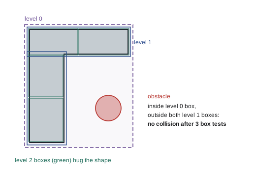
Planning frameworks add a broad phase before the narrow phase: first, cheaply find which pairs of bodies could possibly collide, for example by sorting their bounding boxes along an axis (sweep and prune); then run exact tests only on those pairs. They also maintain an allowed collision matrix listing pairs that never need checking, such as adjacent links that always touch at their joint, or links that cannot geometrically reach each other. On a 7-joint arm with 8 links, there are 28 link pairs; typically more than half can be disabled, saving a large share of self-collision checks.
Worked problem
Sphere tests
An arm link is approximated by three spheres of radius 0.06 m centered at (0.40, 0.00, 0.50), (0.50, 0.00, 0.50) and (0.60, 0.00, 0.50) m. A box-shaped obstacle has been approximated by a sphere of radius 0.10 m at (0.62, 0.12, 0.55) m. Do any spheres overlap, and what is the clearance?
Show solution
- Distance from the third link sphere: \( \sqrt{0.02^2 + 0.12^2 + 0.05^2} = \sqrt{0.0004 + 0.0144 + 0.0025} = 0.130 \) m.
- Sum of radii: \( 0.06 + 0.10 = 0.16 \) m.
- Since 0.130 < 0.16, they overlap by 0.03 m. (The other two spheres are farther away.)
Answer: The spheres overlap by about 3 cm, so the configuration is reported in collision. Sphere models are conservative, so a finer test might show the real link is clear; the planner can either accept the conservative answer or refine.
The GJK algorithm
For convex shapes, the Gilbert-Johnson-Keerthi (GJK) algorithm, published in 1988, computes whether two shapes intersect and, if not, the distance between them. It works on the Minkowski difference \( A \ominus B = \{a - b\} \): the shapes intersect exactly when this set contains the origin, and their distance equals the distance from the origin to the set. GJK never builds the Minkowski difference. It needs only a support function for each shape, which returns the point of the shape farthest in a given direction: \( s_A(\mathbf{d}) = \arg\max_{a \in A} \mathbf{d} \cdot a \). The support of the difference is \( s_A(\mathbf{d}) - s_B(-\mathbf{d}) \). Starting from any point, GJK builds a simplex (a point, segment, triangle or tetrahedron) of support points, repeatedly moving it toward the origin, and stops when it encloses the origin (collision) or can get no closer (separated, with the distance). It usually converges in a handful of iterations. When shapes do overlap, the expanding polytope algorithm (EPA) extends GJK's final simplex to find the penetration depth and direction, which optimization planners use to push a trajectory out of collision.
Worked problem
Support functions
A box centered at the origin has half-extents (0.3, 0.2, 0.1) m and is axis-aligned. What is its support point in the direction \( \mathbf{d} = (1, -2, 0.5) \)? What is the support point of a sphere of radius 0.15 m centered at (1, 0, 0) in the same direction?
Show solution
- Box: take the half-extent with the sign of each component of d: \( (+0.3, -0.2, +0.1) \).
- Sphere: center plus radius times the unit direction. \( \lVert \mathbf{d} \rVert = \sqrt{1 + 4 + 0.25} = 2.29 \).
- Unit direction: \( (0.437, -0.873, 0.218) \).
- Support: \( (1, 0, 0) + 0.15 \times (0.437, -0.873, 0.218) = (1.066, -0.131, 0.033) \).
Answer: Box: (0.3, −0.2, 0.1). Sphere: about (1.066, −0.131, 0.033). These one-line functions are all GJK needs from each shape.
Signed distance fields
A signed distance field (SDF) stores, for every cell of a grid around the robot, the distance to the nearest obstacle surface: positive outside obstacles, negative inside. It is computed once per scene update from an occupancy grid with a distance transform, in time linear in the number of cells. Afterwards, the distance from any point to the environment is a single lookup, and the gradient, the direction that most quickly increases distance, comes from differences between neighboring cells. For a robot modeled as spheres, the clearance of the whole robot is the minimum over spheres of the field value at the center minus the radius. This is why trajectory optimizers such as CHOMP (lesson 9) represent the robot as spheres and the world as an SDF: costs and gradients for thousands of points per iteration become cheap. The trade-offs are memory (a 2 m cube at 1 cm resolution has 8 million cells) and resolution error of up to about half a cell, which must be covered by the safety margin.
import numpy as np
# 2-D signed distance field on a 4 m x 3 m area at 5 cm resolution with two box obstacles
res = 0.05
xs = np.arange(0, 4, res) + res / 2; ys = np.arange(0, 3, res) + res / 2
X, Y = np.meshgrid(xs, ys)
def box_sdf(cx, cy, hx, hy):
    dx, dy = np.abs(X - cx) - hx, np.abs(Y - cy) - hy
    outside = np.hypot(np.maximum(dx, 0), np.maximum(dy, 0))
    inside = np.minimum(np.maximum(dx, dy), 0)
    return outside + inside
sdf = np.minimum(box_sdf(1.2, 1.5, 0.3, 0.6), box_sdf(2.8, 1.0, 0.4, 0.3))
def lookup(px, py):
    i, j = int(py / res), int(px / res)
    gy, gx = np.gradient(sdf, res)
    return sdf[i, j], np.array([gx[i, j], gy[i, j]])
for p in [(0.5, 1.5), (2.0, 1.5), (2.8, 1.5), (1.3, 1.6)]:
    d, g = lookup(*p)
print("point (%.1f, %.1f): distance %+.2f m, gradient (%.2f, %.2f)" % (p[0], p[1], d, g[0], g[1]))point (0.5, 1.5): distance +0.37 m, gradient (-1.00, 0.00) point (2.0, 1.5): distance +0.44 m, gradient (-0.80, 0.51) point (2.8, 1.5): distance +0.22 m, gradient (0.00, 1.00) point (1.3, 1.6): distance -0.17 m, gradient (1.00, 0.00)
Checking motions, not just configurations
Planners must ensure that the motion between two configurations is free, not only its endpoints. Discrete checking samples configurations along the motion, as in lesson 6, at a resolution chosen so that no part of the robot moves farther between samples than the safety margin; if the margin is m and the largest displacement of any point is D, then about \( D/m \) samples are needed. This is simple and widely used, but a thin obstacle can be missed if the resolution is too coarse. Continuous collision detection (CCD) instead computes whether the swept volume of the motion intersects any obstacle, or the first time of contact. Conservative advancement is a common CCD method: compute the current distance d to the nearest obstacle, bound the maximum speed of any point on the robot, and advance in time by the amount guaranteed not to close the gap, repeating until the motion completes or the distance falls below a tolerance. FCL supports both approaches.
Worked problem
Conservative advancement
A robot point moves along a straight motion of length 1.0 m. At the start, its distance to the nearest obstacle is 0.30 m. Taking steps equal to the current distance, and assuming the obstacle distance falls by the distance traveled in the worst case, how many steps does conservative advancement take, and is a 0.05 m tolerance reached before the end?
Show solution
- Step 1: advance 0.30 m; now at 0.30 m along. Suppose the new distance is 0.25 m.
- Step 2: advance 0.25 m to 0.55 m. Suppose the new distance is 0.22 m.
- Step 3: advance 0.22 m to 0.77 m. Suppose the new distance is 0.28 m.
- Step 4: advance 0.23 m to the end at 1.00 m.
Answer: Four distance queries certify the whole motion as free. Discrete checking at a 0.05 m margin would have needed about 20. Conservative advancement takes big steps where clearance is large and small ones near obstacles.
Margins, padding and uncertainty
Geometric checks are exact for the models, but the models are not the robot. Encoder errors, link deflection, calibration errors in the robot base, perception errors in obstacle positions and controller tracking error all mean the real robot may be several centimeters from where the planner thinks it is. Planners therefore pad the robot's collision shapes or inflate obstacles by a margin that covers these errors, often 1 to 5 cm for arms in structured cells and more near people or uncertain perception. Too small a margin causes collisions; too large a margin closes the gaps the robot needs, such as reaching into a bin. Contact tasks, like inserting a peg, need the opposite: the planner must allow specific contacts by disabling checks between the gripper and the object it is grasping, which the allowed collision matrix handles.
Worked problem
Building a margin budget
An arm cell has these error sources at the tool: joint encoder and kinematic calibration 4 mm, tracking error at full speed 6 mm, camera-based obstacle localization 8 mm, and table position uncertainty 3 mm. Using a root-sum-square combination and a safety factor of 2, what margin should the planner add?
Show solution
- Root sum of squares: \( \sqrt{4^2 + 6^2 + 8^2 + 3^2} = \sqrt{16 + 36 + 64 + 9} = \sqrt{125} = 11.2 \) mm.
- With a safety factor of 2: about 22 mm.
Answer: About 22 mm. Adding the errors linearly would give 21 mm before the factor and 42 mm after, which could block reaching into tight spaces; root-sum-square treats the independent errors more realistically.
Common mistakes
MistakeUsing the detailed visual mesh for collision checking
InsteadUse simplified convex hulls, capsules or spheres; they are faster and smoother.
MistakeForgetting objects attached to the gripper
InsteadAdd grasped objects to the robot's collision model so they are checked as it moves.
MistakeChecking every link pair, including ones that cannot collide
InsteadUse an allowed collision matrix to disable impossible or always-touching pairs.
MistakeSampling motions too coarsely
InsteadChoose the step so no point moves farther than the safety margin between checks, or use continuous checking.
MistakePlanning with zero margin
InsteadPad for calibration, tracking and perception errors.
Summary and key terms
- Collision checking dominates planning time, so its speed and correctness are central.
- Robots and worlds are modeled with simplified shapes: spheres, capsules, convex hulls, meshes and octrees.
- Bounding volumes and hierarchies reject far-apart pairs cheaply; broad and narrow phases and allowed collision matrices cut the work further.
- GJK tests convex shapes for intersection and distance using only support functions; EPA gives penetration depth.
- Signed distance fields give constant-time distances and gradients, ideal for trajectory optimization.
- Motions are checked by fine sampling or continuous methods such as conservative advancement.
- Margins must cover calibration, tracking and perception errors without closing needed gaps.
- Collision checker
- Software that tests whether configurations or motions are free of collisions.
- Bounding volume
- A simple shape enclosing a complex one for fast rejection tests.
- BVH
- A bounding-volume hierarchy that recursively splits a shape.
- Broad phase
- A cheap step that finds which pairs could possibly collide.
- Allowed collision matrix
- A list of body pairs that are not checked.
- Support function
- A function returning a shape's farthest point in a given direction.
- GJK
- An algorithm for intersection and distance between convex shapes.
- EPA
- An algorithm that finds penetration depth from GJK's final simplex.
- Signed distance field
- A grid of distances to the nearest surface, negative inside obstacles.
- Conservative advancement
- Continuous checking that steps by the distance guaranteed safe.
Practice problems
Work each problem on paper first, then reveal the answer to check.
What share of sampling-planner time does collision checking often take?
Show answer
About 70 to 90 percent.
Two spheres of radii 0.1 and 0.2 m have centers 0.25 m apart. Do they collide?
Show answer
Yes; 0.25 < 0.3.
What does GJK need from each shape?
Show answer
A support function.
When do two convex shapes intersect, in terms of the Minkowski difference?
Show answer
When it contains the origin.
What does EPA compute?
Show answer
Penetration depth and direction.
Memory for a 1 m cube SDF at 1 cm?
Show answer
One million cells.
How is an SDF gradient obtained?
Show answer
From differences between neighboring cells.
Largest displacement 0.4 m, margin 2 cm: how many samples?
Show answer
About 20.
Why disable adjacent-link pairs?
Show answer
They always touch at the joint and cannot collide in a meaningful way.
Root-sum-square of 3, 4 and 12 mm?
Show answer
13 mm.
Lesson quiz · 5 questions
Score 60% or more to complete this lesson.
Create a free account to save your progress, take quizzes and earn a certificate.