
ROB-350 · Lesson 11 of 12 · 35 min
Planning for manipulators and dynamic environments
Two settings stretch the methods of earlier lessons in different directions. Manipulators live in high-dimensional joint spaces, where sampling and optimization dominate, but their tasks are specified in the Cartesian space of the gripper: reach this grasp, keep the tool level, move along this line. Mobile robots among people and other robots face the opposite difficulty: the configuration space may be small, but obstacles move, so a plan that was valid a second ago may not be now. This lesson covers both. It explains joint-space versus task-space planning, how goals are given through inverse kinematics, how a modern arm planning pipeline such as MoveIt 2 with OMPL is organized, and how grasping shapes the plan. It then turns to dynamic environments: velocity obstacles, the dynamic window approach, model predictive local planners and, briefly, planning under uncertainty in belief space.
Joint space and task space
An arm can be planned in joint space, where the configuration is the vector of joint angles, or in task space, where it is the pose of the end effector. Joint space is where collision checking and joint limits are natural, and where sampling planners work, since every sample is a valid arm configuration; but a straight line in joint space produces a curved, sometimes surprising motion of the gripper. Task space is where the job is defined, and straight-line Cartesian motions are what users expect for approaching a grasp or inserting a part; but a Cartesian path must be converted to joint motions by inverse kinematics at every point, which can fail near singularities or joint limits, or flip between solutions. Most systems combine them: free-space transfers between distant poses are planned in joint space, and short approach, retreat and insertion moves are planned as Cartesian paths.
Worked problem
Where a joint-space line goes
A two-link planar arm with links 1.0 m and 0.8 m moves in joint space from \( (\theta_1, \theta_2) = (0^{\circ}, 90^{\circ}) \) to \( (90^{\circ}, 0^{\circ}) \) along a straight line. Where is the end effector at the start, midpoint and end, and is its path straight?
Show solution
- Start: \( x = 1.0\cos 0 + 0.8\cos 90^{\circ} = 1.0 \), \( y = 0 + 0.8\sin 90^{\circ} = 0.8 \): (1.0, 0.8).
- Midpoint (45°, 45°): \( x = 1.0\cos 45^{\circ} + 0.8\cos 90^{\circ} = 0.707 \), \( y = 0.707 + 0.8 = 1.507 \): (0.71, 1.51).
- End (90°, 0°): \( x = 0 \), \( y = 1.0 + 0.8 = 1.8 \): (0, 1.8).
- The straight line from (1.0, 0.8) to (0, 1.8) passes through (0.5, 1.3) at its midpoint, but the actual midpoint is (0.71, 1.51).
Answer: The end effector bulges about 0.3 m away from the straight Cartesian line. That is harmless in open space but matters near a shelf, which is why approach moves are planned in Cartesian space.
Goals from inverse kinematics
Users specify goals for the gripper, not the joints, so the planner must turn a target pose into joint configurations. A 6-joint arm typically has up to 8 or 16 inverse kinematics solutions for a reachable pose (elbow up or down, wrist flipped, shoulder left or right), and a 7-joint arm has infinitely many, a one-dimensional family parametrized by the elbow angle. Choosing the wrong one can make the plan long or impossible. Planners therefore sample several IK solutions, discard those in collision or beyond joint limits, and either plan to the one closest to the current configuration or plan to several at once and keep the best. Goals are often regions rather than points: any grasp within 10° of vertical around a cylinder, or any placement on a shelf. Goal-region sampling feeds IK solutions for random poses in the region to the planner, which is one reason sampling planners suit arms so well.
Worked problem
Choosing among IK solutions
For a target pose, IK returns four collision-free solutions whose maximum joint difference from the current configuration is 0.4, 1.9, 2.6 and 3.1 rad. The arm's slowest joint moves at 1.2 rad/s. Ignoring obstacles, roughly how long would a direct joint move to each take, and which should the planner try first?
Show solution
- Joint moves are limited by the joint with the largest change: time ≈ largest change ÷ speed.
- 0.4/1.2 = 0.33 s; 1.9/1.2 = 1.6 s; 2.6/1.2 = 2.2 s; 3.1/1.2 = 2.6 s.
- Try the first solution first, and fall back to others if planning fails.
Answer: About 0.3, 1.6, 2.2 and 2.6 s. Picking the nearest IK solution usually gives the shortest, most predictable motion, and keeps the arm from flipping its wrist or elbow unnecessarily.
The MoveIt 2 and OMPL pipeline
MoveIt 2, the main open-source manipulation framework for ROS 2, organizes arm planning as a pipeline. A motion plan request gives the planning group (which joints), the goal as joint values, a pose or constraints, any path constraints such as keeping an orientation, and limits on planning time and attempts. The planning scene supplies the robot model, its current state, the collision environment and attached objects. Request adapters run before planning, for example fixing a start state that is marginally in collision or adding default workspace bounds. The planner plugin, most often OMPL with RRT-Connect, finds a joint-space path. Response adapters then post-process it: smoothing, adding time parametrization with velocity and acceleration limits (time-optimal trajectory generation), and validating the result. Alternatives such as the Pilz industrial motion planner (for deterministic point-to-point, linear and circular moves), CHOMP and STOMP, and the Cartesian path interface plug into the same pipeline. MoveIt Task Constructor chains stages, such as approach, grasp, lift and place, each with its own planner, into a single task.
# MoveIt 2 (Python API, moveit_py) sketch of a pick approach: joint-space transfer, then a Cartesian approach.
# Listing only; requires a robot description, a running MoveIt 2 setup and the moveit_py package.
from moveit.planning import MoveItPy
from geometry_msgs.msg import PoseStamped

robot = MoveItPy(node_name="pick_demo")
arm = robot.get_planning_component("manipulator")

pre_grasp = PoseStamped()
pre_grasp.header.frame_id = "base_link"
pre_grasp.pose.position.x, pre_grasp.pose.position.y, pre_grasp.pose.position.z = 0.55, 0.10, 0.30
pre_grasp.pose.orientation.x, pre_grasp.pose.orientation.y = 1.0, 0.0     # tool pointing down
pre_grasp.pose.orientation.z, pre_grasp.pose.orientation.w = 0.0, 0.0

arm.set_start_state_to_current_state()
arm.set_goal_state(pose_stamped_msg=pre_grasp, pose_link="tool0")
plan = arm.plan()                     # OMPL (e.g. RRTConnect) + smoothing + time parametrization
if plan:
    robot.execute(plan.trajectory, controllers=[])
# The final 10 cm approach is then planned as a straight Cartesian path to the grasp pose.
Grasping and approach
Grasping turns a single goal into a small sequence. The grasp pose itself is usually chosen by a separate grasp planner or learned model (ROB-400 covers grasping in depth). The motion planner must then reach a pre-grasp pose a few centimeters back along the approach direction, move straight in, close the gripper, attach the object to the robot model so it is collision-checked during the next motion, lift straight out to a retreat pose, and plan the transfer. During the final approach the gripper must be allowed to come close to, and eventually touch, the object, so the allowed collision matrix is adjusted for that phase. Many failed picks in practice come not from the main planner but from these transitions: an approach direction blocked by a bin wall, an IK solution that cannot move straight in, or forgetting to attach the object so the arm swings it into a shelf.
Moving obstacles and velocity obstacles
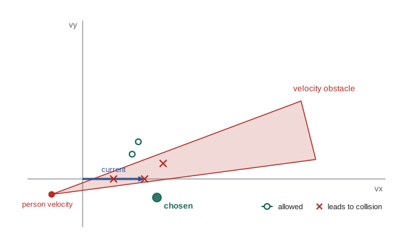
When obstacles move, a path that is collision-free against a snapshot of the world can lead into a collision later. The simplest response is to replan frequently, but planning must then account for where obstacles will be. The velocity obstacle (Fiorini and Shiller, 1998) captures this for local avoidance: for a robot and a moving obstacle, both modeled as discs, the velocity obstacle is the set of robot velocities that would lead to a collision within a time horizon, assuming the obstacle keeps its current velocity. Geometrically it is a cone in velocity space, apex at the obstacle's velocity, containing all relative velocities that point at the combined disc. The robot chooses a velocity outside every velocity obstacle, preferably close to its desired velocity. Reciprocal velocity obstacles and ORCA (optimal reciprocal collision avoidance, van den Berg and colleagues, 2011) assume that other agents share the avoidance effort, which prevents oscillation between robots using the same method and is widely used for robot fleets and crowd simulation.
Worked problem
Time to collision
A robot at (0, 0) moves at (1.0, 0) m/s. A person at (6, 1.5) m walks at (−0.5, −0.25) m/s. Both are modeled as discs, the combined radius being 0.7 m. Will they collide within 10 s if neither changes velocity, and when is their closest approach?
Show solution
- Relative position of the person: p = (6, 1.5). Relative velocity: \( v = (-0.5 - 1.0, -0.25 - 0) = (-1.5, -0.25) \).
- Closest approach time: \( t^* = -\dfrac{p \cdot v}{v \cdot v} = -\dfrac{-9 - 0.375}{2.25 + 0.0625} = \dfrac{9.375}{2.3125} = 4.05 \) s.
- Separation then: \( p + t^* v = (6 - 6.08, 1.5 - 1.01) = (-0.08, 0.49) \), distance 0.50 m.
- 0.50 m is less than 0.7 m, so they collide, shortly before 4 s.
Answer: Yes. Their closest approach, 0.50 m at about 4 s, is inside the combined radius, so the robot's current velocity is in the velocity obstacle and it must slow, speed up or turn.
Dynamic window and MPC local planners
Mobile robots usually split planning into a global planner on the cost map, replanned at about 1 Hz, and a local planner or controller running at 10 to 50 Hz that follows the global path while avoiding obstacles the global plan did not foresee. The dynamic window approach (DWA; Fox, Burgard and Thrun, 1997) samples linear and angular velocities that the robot can reach within one control period given its acceleration limits (the dynamic window), simulates each for a short horizon, discards those that collide, and scores the rest by progress toward the goal, clearance and speed. Model predictive control generalizes this: at each step, optimize a sequence of controls over a horizon of one to a few seconds, subject to the dynamics, velocity and acceleration limits and collision constraints with predicted obstacle positions, apply the first control and repeat. Nav2's Model Predictive Path Integral (MPPI) controller samples thousands of control sequences on the processor and weights them by cost, in the spirit of STOMP (lesson 9). Timed Elastic Bands optimize a short trajectory as a band of timed poses. All of these are local: they can get stuck behind a large obstacle, which is why they follow a global plan.
Worked problem
The dynamic window
A robot moving at v = 0.6 m/s and ω = 0.2 rad/s has acceleration limits 0.5 m/s² and 1.0 rad/s², speed limits 0 to 1.0 m/s and ±1.5 rad/s, and a control period of 0.2 s. What is its dynamic window?
Show solution
- Linear velocity range: \( 0.6 \pm 0.5 \times 0.2 = 0.6 \pm 0.1 \), so 0.5 to 0.7 m/s (within limits).
- Angular velocity range: \( 0.2 \pm 1.0 \times 0.2 = 0.2 \pm 0.2 \), so 0.0 to 0.4 rad/s.
- Sampling, say, 7 by 9 values in this window gives 63 candidate velocity pairs to simulate and score.
Answer: v from 0.5 to 0.7 m/s and ω from 0 to 0.4 rad/s. Only velocities the robot can actually reach next period are considered, which keeps the local plan dynamically feasible.
| Method | Moving obstacles | Horizon | Typical rate | Notes |
|---|---|---|---|---|
| Global replanning (A*, lattice) | Snapshot only | Whole route | 1 Hz | Optimal on the map; slow to react |
| Velocity obstacles / ORCA | Constant-velocity prediction | A few seconds | 10–50 Hz | Multi-robot fleets, crowds |
| Dynamic window approach | Snapshot, re-evaluated | About 1–3 s | 10–20 Hz | Simple, respects acceleration limits |
| MPC / MPPI | Predicted trajectories | 1–3 s | 20–50 Hz | Handles dynamics and constraints |
| Belief-space planning | Uncertain predictions | Varies | Offline or slow | Accounts for sensing uncertainty |
Planning under uncertainty
Everything so far assumed the robot knows its own state and the obstacles' positions exactly, or at least well enough that a safety margin covers the error. When uncertainty is large, as for a robot localized with a particle filter in a featureless corridor (ROB-310 and ROB-340) or a person whose next move is unpredictable, planners can reason about it directly. Chance-constrained planning requires the probability of collision to stay below a threshold, for example by inflating obstacles by a multiple of the position standard deviation. Belief-space planning treats the robot's probability distribution over its state as the thing being planned: a path that passes near distinctive landmarks may be longer but keep the robot well localized, and therefore safer, than a shorter path through a featureless area. The full problem is a partially observable Markov decision process (POMDP) and is intractable in general, but approximate methods, such as planning with Gaussian beliefs propagated by a Kalman filter, are used in practice for navigation and grasping under uncertainty.
Worked problem
A chance constraint as inflation
A robot's lateral position error is Gaussian with standard deviation 0.08 m. The planner must keep the probability of touching a wall below 0.1 percent when passing it. How much extra clearance is needed?
Show solution
- A one-sided probability of 0.001 corresponds to about 3.09 standard deviations.
- Extra clearance: \( 3.09 \times 0.08 = 0.25 \) m.
Answer: About 0.25 m beyond the geometric margin. If localization improves to 0.03 m, the same constraint needs only 0.09 m, so better localization directly opens up narrower passages.
Common mistakes
MistakePlanning approach moves in joint space near clutter
InsteadUse Cartesian paths for short approach and retreat moves where straight-line behavior matters.
MistakeTaking the first IK solution returned
InsteadSample several, check collisions and limits, and prefer the one nearest the current configuration.
MistakeForgetting to attach a grasped object to the robot model
InsteadAttach it so the next motion checks it against the world.
MistakeUsing only a global planner among moving people
InsteadAdd a local planner or MPC that reacts at 10 Hz or faster.
MistakeTreating predicted obstacle positions as certain
InsteadInflate with uncertainty or use chance constraints.
Summary and key terms
- Arms are planned in joint space for free motion and in task space for approach, retreat and constrained moves.
- Goals given as poses or regions are turned into joint configurations by sampling inverse kinematics solutions.
- MoveIt 2 chains request adapters, a planner plugin such as OMPL's RRT-Connect, and smoothing and time parametrization.
- Grasps need pre-grasp, approach, attach, retreat and transfer stages, with collision rules changed for contact.
- Velocity obstacles and ORCA choose velocities that avoid moving agents assuming constant velocities.
- DWA, MPC and MPPI local planners react at high rates within dynamic limits while following a global plan.
- Chance constraints and belief-space planning account for uncertainty in state and predictions.
- Joint space
- The space of an arm's joint angles.
- Task space
- The space of end-effector poses.
- Cartesian path
- A path along which the end effector follows a specified line or curve.
- Goal region
- A set of acceptable goal poses rather than a single pose.
- Planning scene
- MoveIt's model of the robot, its state and its collision environment.
- Pre-grasp pose
- A pose offset from the grasp along the approach direction.
- Velocity obstacle
- The set of velocities leading to collision with a moving obstacle within a horizon.
- ORCA
- Reciprocal collision avoidance in which agents share the avoidance effort.
- Dynamic window approach
- A local planner sampling velocities reachable within one control period.
- Belief-space planning
- Planning over probability distributions of the robot's state.
Practice problems
Work each problem on paper first, then reveal the answer to check.
Why does a straight joint-space move not give a straight gripper path?
Show answer
Forward kinematics is nonlinear.
How many IK solutions does a redundant 7-joint arm have for a reachable pose?
Show answer
Infinitely many.
Which planner is MoveIt 2's usual OMPL default?
Show answer
RRT-Connect.
What must happen to a grasped object before the transfer move?
Show answer
It must be attached to the robot model.
Relative position (4, 0), relative velocity (−1, 0): time to closest approach?
Show answer
4 s.
Where is the apex of a velocity obstacle cone?
Show answer
At the obstacle's velocity.
What does ORCA add to velocity obstacles?
Show answer
Reciprocity: agents share avoidance.
Dynamic window for v = 1.0, a = 0.4, period 0.25 s?
Show answer
0.9 to 1.1 m/s, within limits.
Name a sampling-based MPC controller in Nav2.
Show answer
MPPI.
Extra clearance for σ = 0.05 m at 3.09σ?
Show answer
About 0.15 m.
Lesson quiz · 5 questions
Score 60% or more to complete this lesson.
Create a free account to save your progress, take quizzes and earn a certificate.