Reading and using the psychrometric chart

Raj ran a training session at the Northfield shop every second Thursday, and in January it was psychrometrics. He pinned a large psychrometric chart to the whiteboard, handed out smaller copies, and put a sling psychrometer on the table. "The chart is a map," he told Theo and the two first-year apprentices. "Every point on it is a state of the air. If you know any two properties, you can find the point, and then you can read off all the others. Once you can read it, every process we do with air is a line on that map."

This lesson explains how the chart is built, how to plot and read a state point, how to use it for the quick checks technicians do in the field, and why a chart drawn for sea level gives wrong answers at high elevations.

How the chart is built

The standard psychrometric chart, in the form ASHRAE publishes, has dry-bulb temperature along the bottom and humidity ratio up the right-hand side. Every horizontal line is a line of constant humidity ratio, and so also of constant dew point and vapor pressure. Every vertical line is a line of constant dry bulb. The curved upper boundary is the saturation curve, where relative humidity is 100 %; the dry-bulb, wet-bulb and dew point temperatures are all equal on it, and it rises steeply to the right because warm air can hold much more water than cold air. No real air state lies above it.

The other properties appear as families of lines:

• Relative humidity: curves with the same shape as the saturation curve, below it, usually every 10 %.
• Wet-bulb temperature: straight lines sloping down to the right from the saturation curve, where each wet bulb equals the dry bulb.
• Enthalpy: lines almost parallel to the wet-bulb lines, read from a scale outside the saturation curve. On most charts they are drawn separately from the wet-bulb lines because the two differ slightly.
• Specific volume: steeper lines sloping down to the right, usually every 0.5 ft³/lb.
• Sensible heat ratio: a protractor or half-circle scale in one corner, used in lesson 3 to draw the line along which supply air must lie.

Every chart is drawn for one total pressure. The common ones are for sea level, 29.921 in. Hg (14.696 psia); ASHRAE also publishes charts for higher elevations. The chart is a graph of the same equations lesson 1 used, and software and phone apps do the same calculations without the chart, but the chart shows at a glance how a process moves the air, which no list of numbers does.

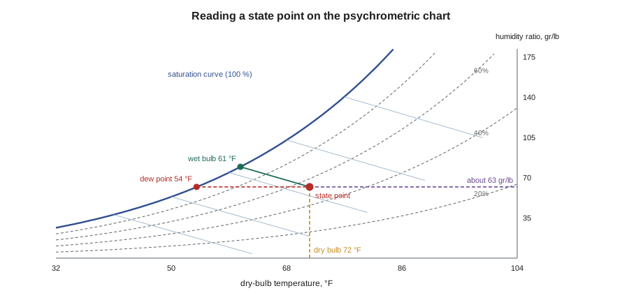
Plotting and reading a state point

Raj had Theo take the sling psychrometer into the produce area of Harvest Lane Market, which had complained of droplets on the misted displays and the glass of the doors. A sling psychrometer has two thermometers, one with a wetted wick; whirled for a minute or two, the wet one settles at the wet-bulb temperature. Theo read 72 °F dry bulb and 61 °F wet bulb. He wet the wick with distilled water first, because tap water leaves minerals that raise the reading, and whirled until two readings in a row agreed.

To plot the point, find 72 °F on the bottom scale and go straight up; find 61 °F on the saturation curve and follow the wet-bulb line down to the right; the point is where they cross. From there:

• Go horizontally right to read the humidity ratio, about 62 to 64 grains per pound.
• Go horizontally left to the saturation curve to read the dew point, about 54 °F.
• Interpolate between the relative humidity curves: about 53 to 54 %.
• Follow the enthalpy lines to the enthalpy scale: about 27 Btu/lb.
• Interpolate between the specific volume lines: about 13.6 ft³/lb on a sea-level chart.

Any two independent properties will do. A dry bulb and a relative humidity from a digital meter, a dry bulb and a dew point, or a wet bulb and a dew point all fix the point. Two properties that move together do not: the dew point and the humidity ratio describe the same thing, so they fix only a horizontal line, not a point.

Field uses of the chart

Raj listed the questions technicians use the chart for most often, all of which the following lessons develop.

• Will this surface sweat? Plot the room air, read the dew point, and compare with the surface temperature, as Theo did for the Novak windows in lesson 1. At Harvest Lane the cold door glass of the frozen-food cases and the misted produce displays were both below the dew point of 54 °F, so the store's anti-sweat heaters and the cases' design had to cope with it.
• What is the coil doing? Plot the air entering and leaving a cooling coil; the change in humidity ratio is the moisture removed and the change in enthalpy is the total heat removed, as the capacity test in RAC-320 lesson 11 showed.
• What happens when two airstreams mix? Mixed air lies on the straight line between them, as lesson 3 shows for outdoor air and return air at the clinic's rooftop unit.
• How much water will a humidifier need to add, or a dehumidifier remove? The change in humidity ratio times the mass flow of air.
• Is the room comfortable? Plot the room state against the comfort zone of lesson 4.

Altitude

Raj's last topic came from a call Northfield had taken the year before. A sister company had asked for help commissioning a packaged unit in Denver, about 5,280 ft above sea level, and the technician who flew out had found the capacity test giving numbers that made no sense. He had used a sea-level chart and the sea-level sensible heat factor.

At higher elevations the total pressure is lower, so for the same vapor pressure the humidity ratio is higher, and for the same dry bulb and wet bulb the air holds more water per kilogram or pound of dry air. More importantly for airflow work, the air is less dense: each cubic foot of air at Denver carries less mass, so it carries less heat for the same temperature change. Fans move volume, not mass, so a fan delivers the same volume at altitude but less mass, and the unit's capacity falls.

The script compares the same pair of readings on a sea-level chart, at Louisville's elevation and at Denver's, and corrects the sensible heat factor for density.

import math
def p_atm(z_m):
    """Standard atmospheric pressure, kPa, at an elevation in meters (feet x 0.3048)."""
    return 101.325 * (1 - 2.25577e-5 * z_m) ** 5.2559
def pws(t):
    """Saturation pressure of water vapor over water, kPa, t in deg C (Magnus form)."""
    return 0.61094 * math.exp(17.625 * t / (t + 243.04))
def w_from_rh(t, rh, p):
    """Humidity ratio, kg of water per kg of dry air."""
    pv = rh * pws(t)
    return 0.622 * pv / (p - pv)
def pv_from_w(w, p):
    return w * p / (0.622 + w)
def dew_point(pv):
    a = math.log(pv / 0.61094)
    return 243.04 * a / (17.625 - a)
def enthalpy(t, w):
    """kJ per kg of dry air."""
    return 1.006 * t + w * (2501 + 1.86 * t)
def spec_volume(t, w, p):
    """Cubic meters per kg of dry air."""
    return 0.287042 * (t + 273.15) * (1 + 1.607858 * w) / p
def wet_bulb(t, w, p):
    """Thermodynamic wet-bulb temperature found by bisection."""
    lo, hi = -40.0, t
    for _ in range(60):
        m = (lo + hi) / 2
        ws = w_from_rh(m, 1.0, p)
        wc = ((2501 - 2.326 * m) * ws - 1.006 * (t - m)) / (2501 + 1.86 * t - 4.186 * m)
        lo, hi = (lo, m) if wc > w else (m, hi)
    return (lo + hi) / 2
def rel_humidity(t, w, p):
    return pv_from_w(w, p) / pws(t)
def c(f): return (f - 32) / 1.8
def f(c_): return c_ * 1.8 + 32
def h_ip(t_c, w):
    """Enthalpy in Btu per lb of dry air (0 deg F datum)."""
    return enthalpy(t_c, w) * 0.4299 + 7.686
GR = 7000   # grains per lb
def w_from_wet_bulb(t, twb, p):
    """Humidity ratio from dry-bulb and wet-bulb readings (psychrometer equation)."""
    ws = w_from_rh(twb, 1.0, p)
    return ((2501 - 2.326 * twb) * ws - 1.006 * (t - twb)) / (2501 + 1.86 * t - 4.186 * twb)

db, wb = 72.0, 61.0            # sling psychrometer readings in the produce area
for name, z_ft in (("sea-level chart", 0), ("Louisville, 460 ft", 460), ("Denver, about 5,280 ft", 5280)):
    P = p_atm(z_ft * 0.3048)
    w = w_from_wet_bulb(c(db), c(wb), P)
    print(f"{name:24s} p={P / 6.895:5.2f} psia  W={w * GR:5.1f} gr/lb  RH={rel_humidity(c(db), w, P):4.0%}  "
          f"dew={f(dew_point(pv_from_w(w, P))):5.1f} F  h={h_ip(c(db), w):5.1f} Btu/lb  v={spec_volume(c(db), w, P) * 16.018:.2f} ft3/lb")
# the sensible heat factor 1.08 Btu/h per cfm per F is density x specific heat x 60 at standard conditions
for name, z_ft in (("Louisville", 460), ("Denver", 5280)):
    factor = 1.08 * p_atm(z_ft * 0.3048) / 101.325
    print(f"sensible factor at {name}: {factor:.2f} Btu/h per cfm per F; 1,000 cfm with a 20 F drop = {factor * 1000 * 20:,.0f} Btu/h")

sea-level chart          p=14.70 psia  W= 62.2 gr/lb  RH= 53%  dew= 54.1 F  h= 27.0 Btu/lb  v=13.59 ft3/lb
Louisville, 460 ft       p=14.45 psia  W= 63.6 gr/lb  RH= 54%  dew= 54.3 F  h= 27.2 Btu/lb  v=13.83 ft3/lb
Denver, about 5,280 ft   p=12.10 psia  W= 79.7 gr/lb  RH= 56%  dew= 55.5 F  h= 29.7 Btu/lb  v=16.58 ft3/lb
sensible factor at Louisville: 1.06 Btu/h per cfm per F; 1,000 cfm with a 20 F drop = 21,243 Btu/h
sensible factor at Denver: 0.89 Btu/h per cfm per F; 1,000 cfm with a 20 F drop = 17,785 Btu/h

At Louisville's 460 ft the error from using a sea-level chart is small: about 1 to 2 grains per pound and under 2 % on the sensible factor. At Denver the humidity ratio is about 17 grains per pound higher than a sea-level chart would show, and the sensible factor falls from 1.08 to about 0.89, so a technician using 1.08 would overestimate the sensible capacity by about 21 %.

The practical rules are simple. Below about 1,000 ft, sea-level charts and factors are fine for field work. At higher elevations, use a chart for the right elevation or software that takes the elevation or the barometric pressure, and multiply the standard air factors by the ratio of local to sea-level pressure. Manufacturers' capacity tables and fan tables are usually for standard air, and their installation manuals give altitude corrections.

Charts, apps and accuracy

Most technicians now use an app or the psychrometric functions built into their digital gauges and meters, which take dry bulb and relative humidity from a probe and display the wet bulb, dew point, enthalpy and humidity ratio. Raj did not object, but he insisted that every apprentice be able to plot a point by hand. The chart shows the shape of a problem; an app shows only its numbers. When a reading looks wrong, the chart makes it obvious: a supply-air reading that plots above the saturation curve, or a coil that seems to add moisture, means a sensor is wet, out of calibration, or in the wrong place.

Accuracy matters most for wet-bulb and humidity readings. A relative humidity sensor accurate to ±2 % gives a wet bulb accurate to a few tenths of a degree, which is fine for comfort work but adds up in a capacity test where small differences are multiplied by large airflows. Readings should be taken where the air is well mixed, away from the coil face and out of direct sunlight, and the sensor given time to settle, especially when moving it between cold supply air and warm return air.

Theo plotted his Harvest Lane readings on the chart, then checked them with the app on his gauges. They agreed to within a gram per kilogram (a few grains per pound). He drew the dew point line across to the left and labeled it: anything colder than that line, in that store, would sweat.