The free electron model revisited: Drude, Sommerfeld and transport

Metals conduct electricity and heat, reflect light, and have a small electronic heat capacity. The simplest model that explains all of these treats the valence electrons as a gas of free particles moving through the volume of the metal, ignoring the ions except as occasional scatterers. PHYS-373 introduced this free-electron gas to compute the Fermi energy and degeneracy pressure. This lesson develops its transport properties: electrical conductivity, the Hall effect, the optical response and thermal conduction. We begin with Paul Drude's classical theory of 1900, which gets surprisingly many things right, and then see how Arnold Sommerfeld's quantum version of 1927 fixes what it gets wrong.

The Drude model

Drude, three years after the discovery of the electron, borrowed the kinetic theory of gases. He assumed that each atom of a metal contributes its valence electrons to a gas of density \(n\), and that these electrons move freely between collisions. Collisions happen randomly with an average time \(\tau\) between them, called the relaxation time, and after each collision an electron emerges with a random velocity, forgetting its previous motion. In an electric field \(\mathbf E\), the average momentum \(\mathbf p\) of an electron obeys

where the second term represents the loss of directed momentum through collisions, like a friction force. In steady state, \(\mathbf p = -e\tau\mathbf E\), so the average drift velocity is \(\mathbf v_d = -e\tau\mathbf E/m\). The current density \(\mathbf j = -ne\mathbf v_d\) is then proportional to the field, which is Ohm's law, \(\mathbf j = \sigma\mathbf E\), with conductivity

Measured resistivities therefore give \(\tau\). For copper at room temperature, \(\rho = 1.68 \times 10^{-8}\ \Omega\,\text{m}\) and \(n = 8.47 \times 10^{28}\ \text{m}^{-3}\) give \(\tau = 2.5 \times 10^{-14}\) s. Drude assumed the electrons collided with the ions and estimated their speed from classical equipartition, \(\tfrac12mv^2 = \tfrac32k_BT\), about 117 km/s at room temperature, giving a mean free path \(\ell = v\tau\) of a few nanometers, comparable to the spacing between atoms. That seemed perfectly reasonable, and it was entirely wrong, for reasons we will see.

The Hall effect

Apply a magnetic field \(\mathbf B\) perpendicular to a current in a thin strip. The Lorentz force pushes the moving charges toward one edge, where they accumulate until the resulting transverse electric field cancels the magnetic force. In steady state, with the current along \(x\) and \(\mathbf B\) along \(z\), the transverse field is \(E_y = R_Hj_xB\), with the Hall coefficient

The striking feature is that \(R_H\) depends only on the density and sign of the carriers, not on \(\tau\). Measuring it counts the carriers. For sodium and copper, the measured Hall coefficients are within about 6 and 30 parts in 100 of the free-electron predictions with one electron per atom, as the program shows, which strongly supports the picture. For aluminum the agreement at room temperature with three electrons per atom is excellent, but at low temperature and high field, aluminum's Hall coefficient changes sign and becomes positive, as if the carriers were positive charges, one per atom. Beryllium, zinc and cadmium also have positive Hall coefficients. No free-electron model can produce a positive sign. The explanation, holes in nearly filled bands, comes from band theory in lessons 9 and 10, and it is one of the strongest pieces of evidence that the lattice matters.

The Hall effect is also a practical tool. Hall sensors in phones measure the Earth's magnetic field to provide a compass, and in cars they detect the angle of camshafts. In two-dimensional electron systems at very low temperature and high field, the Hall resistance becomes quantized in units of \(h/e^2 = 25\,812.807\ \Omega\), the quantum Hall effect discovered by Klaus von Klitzing in 1980, now used to realize the ohm in the SI.

Optical response and the plasma frequency

In an oscillating field \(E(t) = E_0e^{-i\omega t}\), the same equation of motion gives a frequency-dependent conductivity

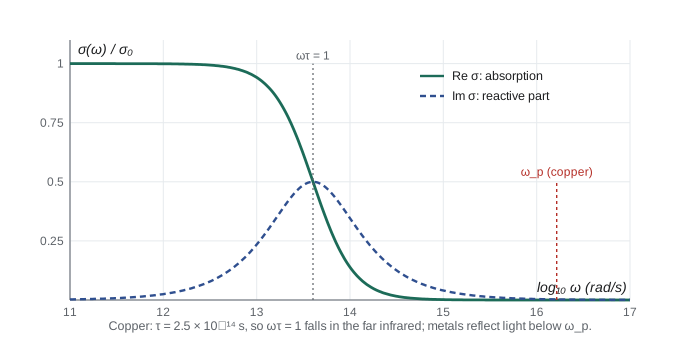
Below \(\omega \sim 1/\tau\), the electrons follow the field and the metal behaves as a resistor. Above it, they cannot keep up, the real (dissipative) part of \(\sigma\) falls as \(1/(\omega\tau)^2\), and the response becomes mainly reactive, like an inductor. Combining \(\sigma(\omega)\) with Maxwell's equations, as in PHYS-382, gives the dielectric function \(\varepsilon(\omega) = 1 - \omega_p^2/\omega^2\) at high frequency, where

is the plasma frequency. Below \(\omega_p\), \(\varepsilon\) is negative, electromagnetic waves cannot propagate and the metal reflects; above it, the metal becomes transparent. For copper, \(\hbar\omega_p = 10.8\) eV, corresponding to a wavelength of 115 nm in the ultraviolet, which is why metals reflect visible light. The alkali metals become transparent in the ultraviolet, close to the free-electron prediction, a discovery made by R. W. Wood in 1933. Copper and gold look colored because transitions of \(d\) electrons absorb part of the visible spectrum, an effect beyond the free-electron model.

Sommerfeld's correction

Drude's theory had one glaring failure. If the conduction electrons were a classical gas, they would contribute \(\tfrac32k_B\) each to the heat capacity, half again as much as the lattice. No such contribution is seen at room temperature. Sommerfeld resolved this in 1927 by replacing the classical distribution with the Fermi–Dirac distribution. As PHYS-373 showed, the electrons fill a Fermi sphere up to an energy \(E_F\) of several eV. Heating to \(T\) can excite only those within about \(k_BT\) of \(E_F\), a fraction of order \(k_BT/E_F\), each gaining about \(k_BT\). The electronic heat capacity is therefore proportional to \(T\):

smaller than the classical value by a factor of order \(k_BT/E_F \approx 1/300\) at room temperature. The precise factor \(\pi^2/2\) comes from the Sommerfeld expansion of integrals over the Fermi function, which PHYS-361 develops. In a metal at low temperature, \(C = \gamma T + \beta T^3\), and the program shows that for copper the two terms are equal at only 3.2 K. Measured \(\gamma\) values exceed the free-electron prediction, 0.695 against 0.503 mJ/(mol K²) for copper, and the ratio defines a thermal effective mass, \(m^*/m = 1.38\), reflecting band structure and electron–phonon interactions. In some compounds containing cerium or uranium, called heavy-fermion metals, \(m^*\) reaches several hundred times \(m\).

Sommerfeld also fixed Drude's mean free path. The electrons that carry current are those at the Fermi surface, moving at the Fermi speed \(v_F = \hbar k_F/m\), about 1600 km/s in copper, more than ten times Drude's thermal speed. With the same \(\tau\), the mean free path is about 40 nm, more than 150 atomic spacings. Electrons do not collide with every ion at all. In a perfect lattice, as Bloch's theorem in lesson 8 will show, an electron wave propagates without any scattering. Resistance comes only from departures from perfect periodicity: lattice vibrations, which dominate at room temperature and give \(\rho \propto T\) above about \(\theta_D/3\), and impurities and defects, which give a temperature-independent residual resistivity. Matthiessen's rule adds the two: \(\rho(T) = \rho_0 + \rho_{ph}(T)\). The residual resistance ratio, \(\rho(300\ \text{K})/\rho(4\ \text{K})\), is a standard measure of a metal's purity; values above 1000 are achieved for carefully refined copper.

import math
# Drude and Sommerfeld models of a metal: Cu, Al and Na.
e, me, hbar, kB = 1.602176634e-19, 9.1093837e-31, 1.054571817e-34, 1.380649e-23
metals = {   # conduction electrons per m^3, resistivity at 295 K (ohm m), measured Hall coefficient (m^3/C)
    'Cu': (8.47e28, 1.68e-8, -5.5e-11),
    'Al': (18.1e28, 2.65e-8, -3.4e-11),
    'Na': (2.65e28, 4.77e-8, -25.0e-11),
}
print("metal  tau (fs)  v_F (km/s)  mean free path (nm)  R_H free-electron  R_H measured")
for name, (n, rho, RH) in metals.items():
    tau = me / (n * e * e * rho)
    vF = hbar * (3 * math.pi ** 2 * n) ** (1 / 3) / me
    print(f"  {name}   {tau * 1e15:7.1f}  {vF / 1e3:10.0f}  {vF * tau * 1e9:19.1f}  {-1 / (n * e):17.2e}  {RH:12.2e}")
print("(classical Drude speed at 295 K would be", f"{math.sqrt(3 * kB * 295 / me) / 1e3:.0f} km/s, giving a path of only a few nm)")
print()
# AC conductivity of copper: sigma(w) = sigma0 / (1 - i w tau)
n, rho = metals['Cu'][:2]
tau = me / (n * e * e * rho); s0 = 1 / rho
eps0 = 8.8541878128e-12
wp = math.sqrt(n * e * e / (eps0 * me))
print(f"copper: sigma0 = {s0:.3e} S/m, tau = {tau:.2e} s, plasma frequency hbar*wp = {hbar * wp / e:.2f} eV "
      f"(lambda_p = {2 * math.pi * 2.998e8 / wp * 1e9:.0f} nm)")
for w in (1e10, 1e12, 1e13, 4e13, 1e14, 1e15):
    sig = s0 / complex(1, -w * tau)
    print(f"  omega = {w:.0e} rad/s: Re sigma/sigma0 = {sig.real / s0:.3f}, Im sigma/sigma0 = {sig.imag / s0:.3f}")
print()
# Sommerfeld: electronic heat capacity gamma T against phonon beta T^3
EF = hbar ** 2 * (3 * math.pi ** 2 * n) ** (2 / 3) / (2 * me)
NA = 6.02214076e23; R = 8.314462618
gamma = math.pi ** 2 / 2 * R * kB / EF          # per mole of electrons, one electron per atom
beta = 12 * math.pi ** 4 / 5 * R / 343.0 ** 3
print(f"copper gamma (free electrons) = {gamma * 1e3:.3f} mJ/mol K^2 (measured 0.695), beta = {beta * 1e3:.4f} mJ/mol K^4")
print(f"electron and phonon terms are equal at T = sqrt(gamma/beta) = {math.sqrt(gamma / beta):.1f} K")
print(f"Wiedemann-Franz: Lorenz number pi^2/3 (kB/e)^2 = {math.pi ** 2 / 3 * (kB / e) ** 2:.3e} W ohm/K^2")

metal  tau (fs)  v_F (km/s)  mean free path (nm)  R_H free-electron  R_H measured
  Cu      24.9        1573                 39.2          -7.37e-11     -5.50e-11
  Al       7.4        2026                 15.0          -3.45e-11     -3.40e-11
  Na      28.1        1068                 30.0          -2.36e-10     -2.50e-10
(classical Drude speed at 295 K would be 116 km/s, giving a path of only a few nm)

copper: sigma0 = 5.952e+07 S/m, tau = 2.49e-14 s, plasma frequency hbar*wp = 10.81 eV (lambda_p = 115 nm)
  omega = 1e+10 rad/s: Re sigma/sigma0 = 1.000, Im sigma/sigma0 = 0.000
  omega = 1e+12 rad/s: Re sigma/sigma0 = 0.999, Im sigma/sigma0 = 0.025
  omega = 1e+13 rad/s: Re sigma/sigma0 = 0.941, Im sigma/sigma0 = 0.235
  omega = 4e+13 rad/s: Re sigma/sigma0 = 0.501, Im sigma/sigma0 = 0.500
  omega = 1e+14 rad/s: Re sigma/sigma0 = 0.139, Im sigma/sigma0 = 0.345
  omega = 1e+15 rad/s: Re sigma/sigma0 = 0.002, Im sigma/sigma0 = 0.040

copper gamma (free electrons) = 0.503 mJ/mol K^2 (measured 0.695), beta = 0.0482 mJ/mol K^4
electron and phonon terms are equal at T = sqrt(gamma/beta) = 3.2 K
Wiedemann-Franz: Lorenz number pi^2/3 (kB/e)^2 = 2.443e-08 W ohm/K^2

Thermal conductivity and the Wiedemann–Franz law

Electrons carry heat as well as charge. Kinetic theory gives \(\kappa = \tfrac13Cv\ell\), the same formula as for phonons in lesson 6. Using Sommerfeld's heat capacity and \(v = v_F\), \(\ell = v_F\tau\), the ratio of thermal to electrical conductivity is

This is the Wiedemann–Franz law, found empirically in 1853 by Gustav Wiedemann and Rudolph Franz, with the Lorenz number calculated by Sommerfeld. Measured values for copper, silver and gold at room temperature are within a few parts in 100 of it. The law explains why good electrical conductors are good thermal conductors, and it fails only when the scattering of heat and charge differ, as at intermediate temperatures where small-angle phonon scattering degrades heat flow more than charge flow. Drude's classical theory happened to give a Lorenz number close to the right value through a cancellation of two large errors, one in the heat capacity and one in the velocity, which is part of why his model was taken seriously for so long.