Case studies and course project

This course has developed electricity and magnetism from charges and fields through potential, Gauss's law and capacitance, to current, circuits and measurement, magnetism, induction and inductance, alternating current, electromagnetic waves and semiconductor devices. Real engineering systems use many of these at once. This lesson works through three case studies: supplying a home electric vehicle charger, transmitting power over long distances, and cleaning industrial exhaust with an electrostatic precipitator. Each shows how a few physical principles, chosen well, answer practical design questions and expose the trade-offs. The lesson then sets out the course project and looks ahead to the courses that build on this one.

Case study 1: a home electric vehicle charger

A Level 2 charger runs from a 240 V circuit (Lesson 9). Suppose it draws a continuous 40 A, so it delivers \(P = VI = 240 \times 40 = 9.6\) kW. The questions an engineer asks: how long will charging take, how thick must the supply cable be, and how much energy is lost on the way?

The cable resistance follows from \(R = \rho L/A\) (Lesson 5), with the current flowing 30 m out and 30 m back. The voltage drop IR reduces the voltage at the charger, and the power \(I^2R\) heats the cable. Electrical codes (the Canadian Electrical Code and the US National Electrical Code) also require the conductors to carry the current without overheating, treat EV chargers as continuous loads sized at 125% of their current, and limit voltage drop, typically to a few percent.

# Level 2 EV charger: 240 V, 40 A continuous, 30 m from the panel (60 m of conductor, out and back)
rho = 1.72e-8 * 1.2          # copper resistivity, ohm m, raised 20% for a warm conductor
V, I, run = 240.0, 40.0, 30.0
for area_mm2 in [6, 10, 16]:
    R = rho * 2 * run / (area_mm2 * 1e-6)
    drop = I * R
    loss = I**2 * R
    print(f"{area_mm2:2d} mm2 copper: R = {R * 1000:5.1f} mohm, drop {drop:4.1f} V ({100 * drop / V:.1f}%), "
          f"loss {loss:5.0f} W ({100 * loss / (V * I):.1f}% of {V * I / 1000:.1f} kW)")

battery_kWh, efficiency = 75.0, 0.90
print(f"Charging {battery_kWh:.0f} kWh at {V * I / 1000:.1f} kW and {efficiency:.0%} efficiency takes {battery_kWh / (V * I / 1000 * efficiency):.1f} h")
print(f"A 150 kW DC fast charger at 400 V supplies {150e3 / 400:.0f} A")

 6 mm2 copper: R = 206.4 mohm, drop  8.3 V (3.4%), loss   330 W (3.4% of 9.6 kW)
10 mm2 copper: R = 123.8 mohm, drop  5.0 V (2.1%), loss   198 W (2.1% of 9.6 kW)
16 mm2 copper: R =  77.4 mohm, drop  3.1 V (1.3%), loss   124 W (1.3% of 9.6 kW)
Charging 75 kWh at 9.6 kW and 90% efficiency takes 8.7 h
A 150 kW DC fast charger at 400 V supplies 375 A

A 6 mm² cable would lose 3.4% of the power and drop 8 V; 10 mm² keeps the drop near 2%; 16 mm² halves the loss again at higher cost. Charging a 75 kWh battery takes almost 9 hours, overnight. A DC fast charger at 150 kW must supply 375 A at 400 V, which is why its cables are thick and often liquid-cooled, and why fast-charging sites need dedicated medium-voltage connections and transformers (Lesson 7). Within the car, the battery's internal resistance (Lesson 6) also heats it during fast charging, so battery management systems taper the current as the battery fills and warms.

Case study 2: why transmit at high voltage?

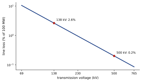
A generating station must send 100 MW to a city 100 km away over a three-phase line whose conductors each have a resistance of 0.05 Ω/km. For three-phase power (Lesson 9), the line current is \(I = P/(\sqrt{3}\,V\cos\phi)\), and the loss is \(3I^2R\).

Higher voltage brings its own physics problems, all from this course. The surface field on the conductors must stay below corona onset (Lesson 3), so high-voltage lines use bundled conductors. Clearances to the ground and to towers must prevent breakdown of the air (Lesson 2). Insulators must withstand both the operating voltage and lightning surges. And the line's inductance and capacitance (Lessons 4 and 8) create reactive power that must be managed, which grows with length. The magnetic field under a line is modest: from Ampère's law (Lesson 7), 418 A at 15 m gives \(\mu_0I/(2\pi r) = 5.6\) µT for a single conductor, about a tenth of the Earth's field, and the fields of the three phases partly cancel.

Case study 3: an electrostatic precipitator

Cement kilns, pulp mills, smelters and biomass boilers emit fine dust that harms health. An electrostatic precipitator removes it using nothing but electric fields. Flue gas passes between grounded collecting plates and fine discharge wires held at tens of kilovolts negative. The very high field near the thin wires (Lesson 3) produces a corona that fills the space with negative ions; the ions stick to dust particles and charge them; and the electric field between wire and plate (Lesson 2) drives the charged particles to the plates, where they are periodically knocked off into hoppers.

The overall collection efficiency is estimated by the Deutsch equation, \(\eta = 1 - e^{-wA/Q}\), where w is the migration velocity, A the total collecting plate area and Q the gas flow rate. With w = 0.09 m/s, Q = 300 m³/s and A = 10 000 m², \(wA/Q = 3.0\) and η = 95%; doubling the plate area raises it to 99.75%. Because efficiency depends exponentially on area, the last fraction of a percent is expensive, and precipitators are often among the largest structures at an industrial plant. Their performance also depends on the electrical resistivity of the dust, which controls how charge leaks away on the plates.

The method behind the case studies

The three studies followed the same pattern:

• Identify the physical quantities that matter: current and resistance for heating, voltage for losses, field strength for breakdown and particle motion.
• Choose the simplest model that captures them: Ohm's law and I²R, three-phase power formulas, Coulomb force against Stokes drag.
• Check against limits set by physics and by codes: breakdown fields, voltage drop limits, conductor ampacity, emission standards.
• Explore the trade-offs: thicker cable against cost, higher voltage against insulation and corona, plate area against efficiency.
• Sanity-check orders of magnitude: a charging time, a percentage loss, a drift speed.

The course project

Choose one of the following problems, or propose your own of similar scope with your instructor's approval, and prepare a report with your model, calculations, a measurement or simulation where possible, checks and conclusions.

• Project A: Home electrical design. For a real or hypothetical home, estimate the loads (including an EV charger or heat pump), select conductor sizes for two circuits from first principles (resistance, voltage drop, loss), compare with code requirements, and estimate annual energy use and cost.
• Project B: Measurement and sensing. Build or simulate a sensor circuit (a strain gauge bridge, a thermistor divider or a Hall-effect current sensor), predict its output with the theory of this course, measure or simulate it, and analyze the sources of error including meter loading.
• Project C: Power systems. Compare transmitting a given power over a given distance at several voltages, including resistive loss, corona considerations, conductor and insulation requirements, and the effect of power factor, and recommend a voltage with reasons.
• Project D: Energy storage and conversion. Compare capacitors, batteries and an inductive storage scheme (or a solar module and battery system) for a defined application, using energy, power, efficiency and cost, and recommend a design.

Every report should include circuit or field diagrams, state assumptions and their effect, check units and orders of magnitude, compare at least one result with an independent estimate or measurement, and observe electrical safety in any practical work.

Looking ahead

Electricity and magnetism underpin electrical, computer and much of mechanical and civil engineering. Circuit analysis courses (ELE-202 and ELE-203) develop the methods of Lessons 5, 6 and 9 systematically; electromagnetics extends Gauss's, Faraday's and Ampère's laws to fields and waves in full (MATH-209 lays the mathematical groundwork); electric machines and power systems build on induction, transformers and three-phase power; electronics builds on the semiconductor devices of Lesson 11. For every engineer, the principles of this course explain how the power and information systems they depend on actually work.