Gas well testing and pseudo-pressure

The C-4 deliverability test gave a stabilized line and an AOF, but it did not say why the well performs as it does. Is the formation permeability high and the well damaged, or is the rock poorer than mapped and the completion clean? How much of the apparent skin comes from non-Darcy flow? Pressure transient analysis answers those questions. Farid asks Ethan to design and interpret a two-rate drawdown on C-4 with a downhole gauge, and to set up the same analysis for the long shut-ins planned in the Marcellus wells. “The equations are the oil equations,” he says, “once you put the gas in the right variables.”

Why gas needs special variables

The diffusivity equation for slightly compressible liquids is linear because the fluid's viscosity and compressibility are nearly constant. For gas, both change strongly with pressure, and density is proportional to p/z. Writing the continuity equation and Darcy's law for a real gas gives:

The equation is nonlinear because μ, z and c_t depend on p. Al-Hussainy, Ramey and Crawford (1966) removed most of the nonlinearity by defining the real-gas pseudo-pressure:

Written in m(p), the left side of the gas diffusivity equation becomes the same as the liquid equation. The right side still contains μc_t, which varies with pressure, but for drawdowns and buildups of moderate size, evaluating it at the initial or average pressure is accurate. Pseudo-time, defined by Agarwal (1979) with μc_t inside a time integral, handles the remaining nonlinearity when pressures change a lot, as in long tests in tight rock. With these substitutions, every solution of the liquid diffusivity equation, every type curve and every derivative plot carries over to gas.

Pseudo-pressure has awkward units, psi²/cp, but it is easy to compute: integrate p/(μz) numerically from the gas property table of Lesson 2. At low pressure, where μz is roughly constant, m(p) is proportional to p², which is why the pressure-squared equations of Lesson 5 work there. At high pressure, where p/(μz) is roughly constant, m(p) is linear in p. In between, only m(p) is exact.

Drawdown and buildup analysis

In infinite-acting radial flow, after wellbore storage has ended and before the boundaries are felt, the flowing pseudo-pressure falls linearly with the logarithm of time. In field units, with q in Mscf/d and T in °R:

The slope of m(p_wf) against log t on a semilog plot, m', gives the permeability-thickness product: kh = 1637 qT/m'. The value on the straight line at one hour gives the apparent skin s'. Buildup analysis uses Horner time, (t_p + Δt)/Δt, in exactly the same way, with the extrapolated pseudo-pressure at Horner time 1 giving m(p*) and from it an estimate of average pressure. The apparent skin from a gas test is the sum of the mechanical skin s, from damage, partial penetration or stimulation, and the rate-dependent skin D q:

A single test cannot separate the two. Two tests at different rates can: plotting s' against q gives a straight line with intercept s and slope D. This is the most important practical result of gas well testing, because the remedies differ completely. Mechanical damage can be removed with an acid or a refracture; non-Darcy skin is reduced by spreading the flow over more of the formation with more perforations, a longer interval or a fracture.

# Real-gas pseudo-pressure m(p) and a two-rate drawdown test on the C-4 well:
# permeability from the semilog slope, apparent skin at each rate, then true skin and the non-Darcy coefficient D.
import math
SI = False     # True: metric units, False: oilfield units
def sutton(gg):
    return 169.2 + 349.5 * gg - 74.0 * gg ** 2, 756.8 - 131.07 * gg - 3.6 * gg ** 2

def z_dak(Tpr, ppr):
    """Dranchuk-Abou-Kassem z-factor by fixed-point and Newton iteration."""
    A = [0.3265, -1.0700, -0.5339, 0.01569, -0.05165, 0.5475, -0.7361, 0.1844, 0.1056, 0.6134, 0.7210]
    c1 = A[0] + A[1] / Tpr + A[2] / Tpr ** 3 + A[3] / Tpr ** 4 + A[4] / Tpr ** 5
    c2 = A[5] + A[6] / Tpr + A[7] / Tpr ** 2
    c3 = A[8] * (A[6] / Tpr + A[7] / Tpr ** 2)
    def f(z):
        r = 0.27 * ppr / (z * Tpr)
        return z - (1 + c1 * r + c2 * r ** 2 - c3 * r ** 5 + A[9] * (1 + A[10] * r ** 2) * r ** 2 / Tpr ** 3 * math.exp(-A[10] * r ** 2))
    z = 1.0
    for _ in range(100):
        d = (f(z + 1e-7) - f(z)) / 1e-7
        zn = z - f(z) / d
        if abs(zn - z) < 1e-10: return zn
        z = zn
    return z

def mu_lge(T_R, rho_gcc, M):
    K = (9.4 + 0.02 * M) * T_R ** 1.5 / (209 + 19 * M + T_R)
    X = 3.5 + 986 / T_R + 0.01 * M
    return 1e-4 * K * math.exp(X * rho_gcc ** (2.4 - 0.2 * X))

gg, T_R = 0.65, 160 + 459.67; M = 28.966 * gg
Tpc, ppc = sutton(gg)
def props(p):
    z = z_dak(T_R / Tpc, p / ppc)
    rho = p * M / (z * 10.732 * T_R) / 62.428
    return z, mu_lge(T_R, rho, M)
# m(p) = 2 * integral of p / (mu z) dp, by the trapezoid rule in 10 psi steps
P = [0.0]; Mp = [0.0]; f_old = 0.0
for i in range(1, 251):
    p = 10.0 * i; z, mu = props(p); f = p / (mu * z)
    Mp.append(Mp[-1] + (f + f_old) * 10.0); P.append(p); f_old = f
mp = lambda p: Mp[int(p // 10)] + (Mp[int(p // 10) + 1] - Mp[int(p // 10)]) * (p % 10) / 10
def p_of(m):
    i = max(j for j in range(len(Mp)) if Mp[j] <= m)
    return P[i] + 10 * (m - Mp[i]) / (Mp[i + 1] - Mp[i])

conv = 6.894757 ** 2 / 1e6        # converts psi2/cp to MPa2/(mPa.s)
print(" p kPa     m(p) MPa2/(mPa.s)" if SI else " p psia    m(p) psi2/cp")
for pin in ([3500, 7000, 10500, 14000, 14341] if SI else [500, 1000, 1500, 2000, 2080]):
    p = pin * 0.145038 if SI else pin
    print(f"{pin:7,.0f}   {mp(p) * conv:10.1f}" if SI else f"{pin:7,.0f}   {mp(p):12.4e}")

# Synthetic test data from the radial solution (true k 80 mD, h 26 ft, skin 2.0, D 2.5e-4 per Mscf/d)
k, h, phi, rw, S, D, pi = 80.0, 26.0, 0.14, 0.35, 2.0, 2.5e-4, 2080.0
zi, mui = props(pi)
cg = 1 / pi - (z_dak(T_R / Tpc, pi * 1.001 / ppc) - z_dak(T_R / Tpc, pi * 0.999 / ppc)) / (0.002 * pi) / zi
ct = cg * 0.76 + 3e-6 * 0.24 + 4e-6
def pwf(q, t):
    mprime = 1637 * q * T_R / (k * h)
    return p_of(mp(pi) - mprime * (math.log10(t) + math.log10(k / (phi * mui * ct * rw ** 2)) - 3.23 + 0.869 * (S + D * q)))
results = []
for q in (5000.0, 10000.0):                   # Mscf/d
    times = [1, 2, 4, 8, 16]
    data = [(t, round(pwf(q, t), 1)) for t in times]
    # analysis: slope of m(pwf) against log t, then k and the apparent skin S' at this rate
    xs = [math.log10(t) for t, p in data]; ys = [mp(p) for t, p in data]
    n = len(xs); mx, my = sum(xs) / n, sum(ys) / n
    slope = -sum((a - mx) * (b - my) for a, b in zip(xs, ys)) / sum((a - mx) ** 2 for a in xs)
    k_est = 1637 * q * T_R / (slope * h)
    m1 = my + slope * mx                       # m(pwf) at 1 hour on the straight line
    Sp = 1.151 * ((mp(pi) - m1) / slope - math.log10(k_est / (phi * mui * ct * rw ** 2)) + 3.23)
    results.append((q, Sp))
    qq = f"{q * 0.0283168:,.0f} 10^3 m3/d" if SI else f"{q / 1000:.0f} MMscf/d"
    pw = ", ".join(f"{t} h {p / 0.145038:,.0f}" if SI else f"{t} h {p:,.0f}" for t, p in data)
    print(f"Rate {qq}: pwf {pw}")
    print(f"   k = {k_est:.2f} mD, apparent skin S' = {Sp:.2f}")
(q1, s1), (q2, s2) = results
Dfit = (s2 - s1) / (q2 - q1); Sfit = s1 - Dfit * q1
print(f"True skin {Sfit:.2f}; non-Darcy D = {Dfit / 0.0283168:.2e} per (10^3 m3/d)" if SI else
      f"True skin {Sfit:.2f}; non-Darcy D = {Dfit:.2e} per Mscf/d")

 p psia    m(p) psi2/cp
    500     1.9902e+07
  1,000     7.9321e+07
  1,500     1.7554e+08
  2,000     3.0316e+08
  2,080     3.2603e+08
Rate 5 MMscf/d: pwf 1 h 2,008, 2 h 2,005, 4 h 2,003, 8 h 2,000, 16 h 1,998
   k = 80.00 mD, apparent skin S' = 3.26
Rate 10 MMscf/d: pwf 1 h 1,915, 2 h 1,909, 4 h 1,904, 8 h 1,899, 16 h 1,893
   k = 79.84 mD, apparent skin S' = 4.48
True skin 2.04; non-Darcy D = 2.44e-04 per Mscf/d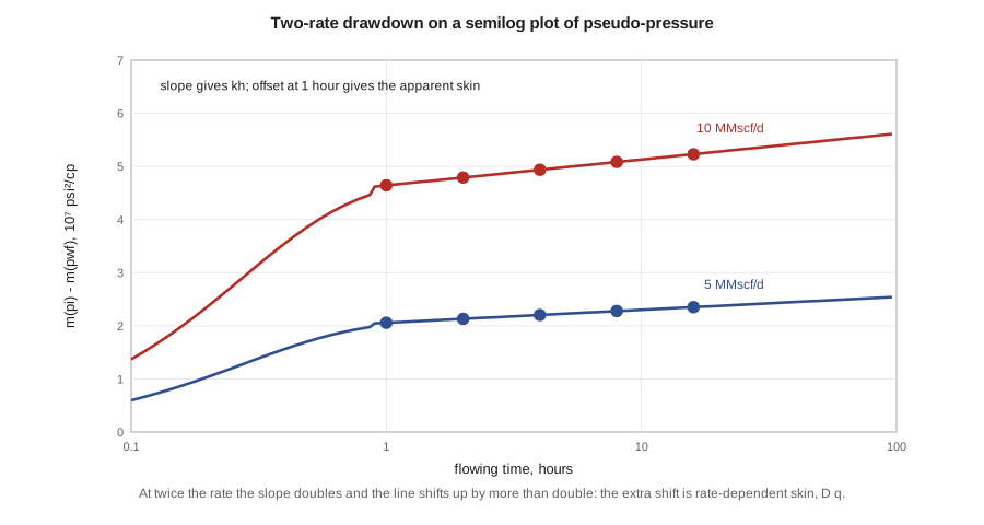

The analysis recovers a permeability of 80 mD for the 26-ft net interval, an apparent skin of about 3.3 at the lower rate and 4.5 at the higher rate, a mechanical skin of 2.0 and a non-Darcy coefficient of about 2.4 × 10⁻⁴ per Mscf/d. At 10 MMscf/d, the non-Darcy term contributes a skin of about 2.4, more than the mechanical damage. That matches the LIT result of Lesson 5, where about a fifth of the drawdown went into non-Darcy flow. Ethan's recommendation follows: a small acid wash would remove part of the mechanical skin, but adding perforations over the full net interval, which the original completion left partly unperforated, would cut both terms.

The derivative plot and flow regimes

Modern test interpretation relies on the log-log plot of the pseudo-pressure change and its derivative with respect to the logarithm of time, introduced by Bourdet in 1983. Each flow regime has a signature. Wellbore storage gives a unit slope on both curves at early time. Infinite-acting radial flow gives a flat derivative, whose level gives kh. Linear flow, into a fracture or along a channel, gives a half slope; bilinear flow, in a finite-conductivity fracture, a quarter slope. A closed boundary gives a late unit slope in drawdown and a falling derivative in buildup, and a constant-pressure boundary such as a strong aquifer a falling derivative in both. The derivative plot is a diagnostic first and a calculation second: identify the regimes, then apply the right specialized analysis to each.

Testing tight and shale gas wells

In the Marcellus, a conventional test would take far too long. With permeability in the microdarcy range, radial flow around a horizontal well with dozens of fractures would not develop for years. What a Ten Mile Ridge well shows instead is linear flow from the matrix into each hydraulic fracture, often lasting for the first one to five years of production. In linear flow the pseudo-pressure change grows with the square root of time, and the slope of Δm against √t gives the product of fracture face area and the square root of matrix permeability, A√k, not k by itself. That product is what controls the well's early performance.

Because shut-ins are costly in such wells, the industry now interprets the production data itself, a method called rate-transient analysis. The daily rates and flowing pressures from the wellhead, converted to bottomhole conditions, are normalized as rate-normalized pseudo-pressure, Δm/q, and plotted against material balance pseudo-time. The same flow regime signatures appear: a half slope for linear flow, then a unit slope when the stimulated region begins to deplete. Rate-transient analysis gives A√k, the end of linear flow and a minimum estimate of the gas in contact with the well. Lesson 8 uses these results to build the type well.

Designing a gas well test

Good tests are designed, not just run. The design sets the gauge type and placement, the flow rates and durations and the shut-in times, from a forward simulation with the best current estimate of the reservoir. Ethan's checklist for C-4 covers several points. Use a downhole gauge with memory, because wellhead pressures in gas wells are affected by liquid in the tubing and temperature changes. Flow long enough at each rate to reach at least one log cycle of radial flow after wellbore storage ends. Choose two rates that differ by at least a factor of two so that D can be resolved. Measure gas, condensate and water rates continuously. Record the separator conditions for the condensate-gas ratio. For sour wells in Pennsylvania, follow the DEP's requirements on flaring and on hydrogen sulfide safety during the test, and conserve the gas into the gathering system wherever possible.