Water influx and abnormally pressured reservoirs

Ethan's p/z analysis of the Oriskany sandstone pool assumed a volumetric tank. Farid is not ready to accept that. The Oriskany sandstone sits on a regional water-bearing sandstone, and the gas-water contact covers most of the pool's base. “Water drive is the most common way a p/z plot lies to you,” he says. “And it lies most convincingly early, when the points still look straight.” The second half of the lesson deals with the opposite case, a reservoir whose pressure is far above hydrostatic, like the Marcellus under the Ten Mile Ridge block. Both break the simple straight line, in different directions.

The general gas material balance

When water flows into the gas zone from an aquifer, the pore volume available to gas shrinks. Adding water influx W_e, produced water W_p and the expansion of connate water and rock to the volumetric balance gives the general gas material balance:

The left side is the reservoir volume of everything withdrawn. On the right, the first term is the expansion of the remaining gas, the second the expansion of connate water and the shrinkage of pore volume as pressure falls, and the third the water that has entered from the aquifer. For a normally pressured reservoir the middle term is tiny compared with gas expansion, because gas compressibility is a hundred times larger than water or rock compressibility. Water influx, however, can be large.

How water drive bends the p/z plot

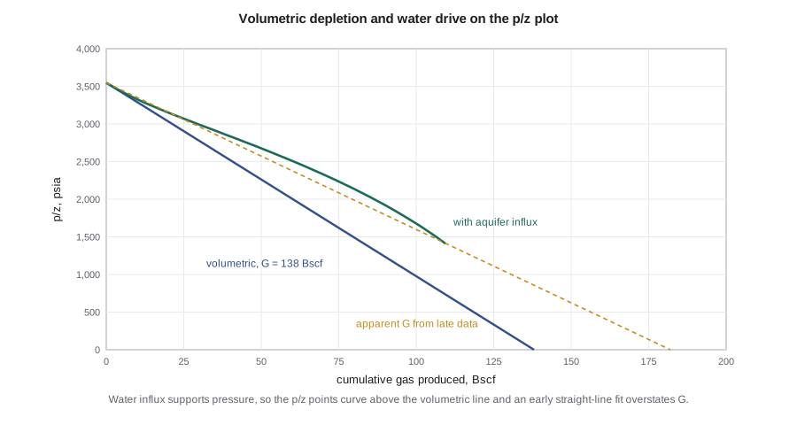
Water influx replaces some of the withdrawn volume, so the pressure falls more slowly than in a volumetric tank. On the p/z plot the points lie above the volumetric line, at first only slightly and then increasingly. In a strong water drive the pressure may barely fall at all. The danger is in the middle ground. With a moderate aquifer, the first few points look almost straight, but their slope is too shallow, and the extrapolation gives a gas in place that is too high. Engineers who book reserves on such a line later find that the water arrives at the wells long before the p/z line said the gas would run out.

Several diagnostics catch water drive earlier than the p/z plot. The Cole plot, borrowed from oil material balance, plots F/E_g, the reservoir withdrawal divided by the gas expansion per unit of gas in place, against cumulative production. For a volumetric reservoir F/E_g is constant and equals G; with water influx it rises with time. The Havlena-Odeh form of the balance, F = G E_g + W_e, plotted as F/E_g against W_e/E_g for an assumed aquifer model, gives a straight line with intercept G and slope 1 when the aquifer model is right. Rising water-gas ratios at structurally low wells, and pressure gauges in observation wells in the aquifer, are direct evidence.

Aquifer models

Water influx is calculated with an aquifer model that relates the influx to the pressure history at the gas-water contact. The pot aquifer, the simplest, assumes the aquifer is small and in instant pressure equilibrium with the reservoir, so W_e = (c_w + c_f) W_i Δp, where W_i is the aquifer water volume. It suits small aquifers only. The van Everdingen-Hurst model (1949) solves the radial diffusivity equation for the aquifer and superposes the response to each pressure step at the contact; it is rigorous for an infinite or bounded radial or linear aquifer, but it needs a convolution over the whole pressure history.

Fetkovich's 1971 model is the practical compromise used in most material balance software. It treats the aquifer as a finite tank connected to the reservoir through a productivity index J, and assumes pseudo-steady-state flow from aquifer to reservoir. Over a time step Δt, with average aquifer pressure p̄_a and average reservoir boundary pressure p̄_r:

Here W_ei is the maximum encroachable water, the water that would enter if the aquifer pressure fell from p_i to zero, and the aquifer pressure falls in proportion to the water it has given up. Two parameters, W_ei and J, are fitted to the pressure history. The Fetkovich model reproduces the van Everdingen-Hurst results well for most finite aquifers and is easy to step forward in time.

# Water influx: a gas tank with a Fetkovich aquifer, compared with volumetric depletion,
# and the Ramagost-Farshad correction for an abnormally pressured reservoir.
import math
SI = False     # True: metric units, False: oilfield units
def sutton(gg):
    return 169.2 + 349.5 * gg - 74.0 * gg ** 2, 756.8 - 131.07 * gg - 3.6 * gg ** 2

def z_dak(Tpr, ppr):
    """Dranchuk-Abou-Kassem z-factor by fixed-point and Newton iteration."""
    A = [0.3265, -1.0700, -0.5339, 0.01569, -0.05165, 0.5475, -0.7361, 0.1844, 0.1056, 0.6134, 0.7210]
    c1 = A[0] + A[1] / Tpr + A[2] / Tpr ** 3 + A[3] / Tpr ** 4 + A[4] / Tpr ** 5
    c2 = A[5] + A[6] / Tpr + A[7] / Tpr ** 2
    c3 = A[8] * (A[6] / Tpr + A[7] / Tpr ** 2)
    def f(z):
        r = 0.27 * ppr / (z * Tpr)
        return z - (1 + c1 * r + c2 * r ** 2 - c3 * r ** 5 + A[9] * (1 + A[10] * r ** 2) * r ** 2 / Tpr ** 3 * math.exp(-A[10] * r ** 2))
    z = 1.0
    for _ in range(100):
        d = (f(z + 1e-7) - f(z)) / 1e-7
        zn = z - f(z) / d
        if abs(zn - z) < 1e-10: return zn
        z = zn
    return z

gg, T_R, pi = 0.65, 160 + 459.67, 3100.0
Tpc, ppc = sutton(gg)
z = lambda p: z_dak(T_R / Tpc, p / ppc)
Bg = lambda p: 0.02827 * z(p) * T_R / p / 5.615          # rb/scf
G = 138e9; Bgi = Bg(pi)
Wei, J = 1.5e8, 40.0            # encroachable water (bbl) and aquifer productivity index (bbl/d/psi)
q, dt = 30e6, 91.25             # gas rate scf/d, time step days

def step(p_old, Gp, We_old, pa):
    """Solve G(Bg - Bgi) + We = Gp*Bg for the new tank pressure with a Fetkovich influx step."""
    def resid(p):
        dWe = Wei / pi * (pa - (p_old + p) / 2) * (1 - math.exp(-J * pi * dt / Wei))
        return G * (Bg(p) - Bgi) + We_old + dWe - Gp * Bg(p), dWe
    lo, hi = 100.0, p_old
    for _ in range(80):
        mid = (lo + hi) / 2
        if resid(mid)[0] > 0: lo = mid
        else: hi = mid
    return mid, resid(mid)[1]

rows = []
# volumetric pressure from p/z = (pi/zi)(1 - Gp/G), solved by bisection
def p_volumetric(Gp):
    target = pi / z(pi) * (1 - Gp / G); lo, hi = 50.0, pi
    for _ in range(80):
        mid = (lo + hi) / 2
        if mid / z(mid) > target: hi = mid
        else: lo = mid
    return mid
p_w, We, pa = pi, 0.0, pi
for k in range(1, 41):
    Gp = q * dt * k
    p_new, dWe = step(p_w, Gp, We, pa)
    We += dWe; pa = pi * (1 - We / Wei); p_w = p_new
    if k % 8 == 0: rows.append((k * dt / 365, Gp, p_volumetric(Gp), p_w, We))
f = (lambda v: v / 0.145038) if SI else (lambda v: v)
print(" year  Gp       p/z volumetric  p/z water drive  We" + ("   (kPa, 10^9 m3, 10^6 m3)" if SI else "   (psia, Bscf, MMbbl)"))
for yr, Gp, pv, pw, we in rows:
    g = Gp * 0.0283168 / 1e9 if SI else Gp / 1e9
    w = we * 0.158987 / 1e6 if SI else we / 1e6
    print(f"{yr:5.0f} {g:7.2f}  {f(pv / z(pv)):10,.0f}  {f(pw / z(pw)):12,.0f}  {w:8.2f}")
# apparent gas in place from a straight line through the first and last water-drive points
yr, Gp, pv, pw, we = rows[-1]
Gapp = Gp / (1 - (pw / z(pw)) / (pi / z(pi)))
print(f"Apparent OGIP from the late p/z point: {Gapp * 0.0283168 / 1e9:.2f} x 10^9 m3 (true {G * 0.0283168 / 1e9:.2f})" if SI else
      f"Apparent OGIP from the late p/z point: {Gapp / 1e9:.0f} Bscf (true {G / 1e9:.0f})")

# Abnormal pressure: Ramagost-Farshad correction of p/z with effective compressibility
cw, cf, swi = 3.0e-6, 15e-6, 0.22
ce = (cw * swi + cf) / (1 - swi)
pi2 = 31000 * 0.145038 if SI else 4500.0; Tpc2, ppc2 = sutton(0.74); T2 = 190 + 459.67
z2 = lambda p: z_dak(T2 / Tpc2, p / ppc2)
print(f"Effective compressibility {ce * 145.038:.4f} 1/MPa" if SI else f"Effective compressibility {ce:.2e} 1/psi")
for pin in ([31000, 27500, 24000, 20500] if SI else [4500, 4000, 3500, 3000]):
    p = pin * 0.145038 if SI else pin
    raw = p / z2(p); corr = raw * (1 - ce * (pi2 - p))
    print(f"  p {f(p):7,.0f}  p/z {f(raw):7,.0f}  corrected {f(corr):7,.0f}")

 year  Gp       p/z volumetric  p/z water drive  We   (psia, Bscf, MMbbl)
    2   21.90       2,984         3,120      5.27
    4   43.80       2,422         2,776     15.48
    6   65.70       1,859         2,409     27.72
    8   87.60       1,296         1,974     41.71
   10  109.50         733         1,409     58.28
Apparent OGIP from the late p/z point: 182 Bscf (true 138)
Effective compressibility 2.01e-05 1/psi
  p   4,500  p/z   4,728  corrected   4,728
  p   4,000  p/z   4,364  corrected   4,320
  p   3,500  p/z   3,945  corrected   3,866
  p   3,000  p/z   3,466  corrected   3,362

The code produces the pool at a constant 30 MMscf/d for ten years and solves the material balance at each quarter. With the weak aquifer assumed, the p/z values after two years are only about 5 percent above the volumetric line, well within the scatter of real pressure data. After ten years they are nearly double the volumetric values, and a line through the late points extrapolates to about 182 Bscf, a third more than the true gas in place. By then about 58 million barrels of water has entered the pool.

Ethan reruns the Oriskany sandstone pool history with the Fetkovich model, letting the software fit W_ei and J. The best fit has almost no aquifer: the data cannot distinguish a weak aquifer from none over the first four years. That is the honest conclusion, and he writes it that way: the material balance gas in place is an upper bound until either the p/z plot bends or water appears. He recommends running a pulsed-neutron log in the lowest well every two years to watch for the gas-water contact rising, a cheap way to detect influx years before water is produced.

Effect of water drive on recovery

Water drive reduces the ultimate recovery of most gas reservoirs, which surprises engineers trained on oil, where water drive is the best mechanism. Advancing water bypasses and traps gas at a residual gas saturation of 15 to 40 percent of pore volume, and it traps that gas at high pressure, where each pore volume holds many standard volumes. Wells also water out and stop flowing long before the gas zone is depleted, because gas wells have limited ability to lift water. Recovery under a strong water drive may be only 50 to 70 percent, against 80 to 90 percent for volumetric depletion. Producing a water-drive gas pool fast, so that pressure falls before the water arrives, is often the best strategy, together with placing wells high on structure.

Abnormally pressured gas reservoirs

The Marcellus under the Ten Mile Ridge block is overpressured. Its initial pressure of about 4,500 psia at 7,875 ft corresponds to a gradient of about 0.57 psi/ft, against a normal hydrostatic gradient near 0.44 psi/ft. Overpressure is common in tight gas and shale, where gas generated from organic matter in the rock could not escape fast enough to equilibrate with the surface. It brings several engineering consequences: heavier drilling mud and stronger casing, more gas in place per unit of pore volume and higher initial rates, but also rock that compacts as pressure falls.

In an overpressured reservoir the pore volume compressibility can be much larger than in normally pressured rock, and the middle term of the material balance is no longer negligible. Ignoring it makes the early p/z points fall slowly, just like water influx, and the straight-line extrapolation overstates G, sometimes by 50 percent or more. Classic examples in the Gulf Coast in the 1960s and 1970s led to the corrections now in use. Ramagost and Farshad (1981) wrote the balance with an effective compressibility c_e:

Plotting the corrected p/z against G_p restores the straight line, if c_e is known. When it is not, the corrected line can be found by trying values of c_e until the plot straightens, or c_e can be measured on cores under stress. Some overpressured reservoirs show a distinct two-slope p/z curve, with a shallow early slope while the rock compacts and a steeper later one. The code shows that, for the Marcellus rock compressibility assumed here, the correction is about 3 percent after a 1,000 psi drawdown. That is modest, because the Marcellus is a stiff siltstone, but in soft, highly overpressured sands it can be ten times larger.

For the Ten Mile Ridge wells themselves, the question is mostly academic: average reservoir pressure in the Marcellus is never measured in the classical way, because the rock is too tight for pressure to equalize. The correction matters for the conventional pools and for interpreting the long shut-in pressures that the team does collect in the Marcellus for rate-transient analysis.