Real-gas properties and the z-factor

With the composition in hand, Farid asks Ethan to build the gas property tables that every later calculation will use: the z-factor, the formation volume factor, the density, the viscosity and the compressibility, from the initial reservoir pressure of about 4,500 psia down to the abandonment pressure. “Everything in gas engineering runs through z,” Farid says. “Get it wrong by 5 percent and your gas in place is wrong by 5 percent before you start.”

From the ideal gas law to the real-gas law

An ideal gas obeys pV = nRT exactly. Its molecules occupy no volume and exert no forces on each other. Real gases at reservoir conditions do neither. At moderate pressures, attraction between molecules pulls them closer than the ideal gas law predicts, so the real gas occupies less volume. At high pressures, the finite size of the molecules dominates and the real gas occupies more volume than an ideal gas would. Engineers account for both effects with a single correction, the gas deviation factor or z-factor, defined as the ratio of the real volume to the ideal volume at the same pressure and temperature:

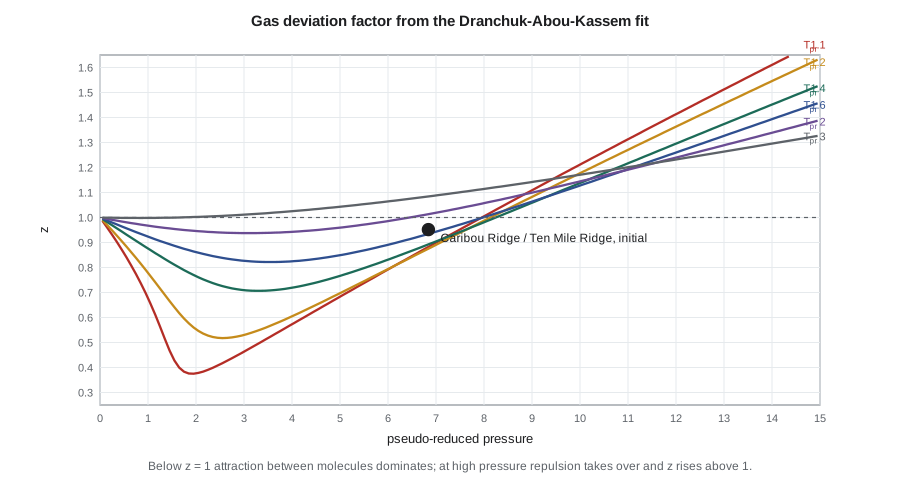
The z-factor is close to 1 at low pressure, falls to a minimum, typically between 0.8 and 0.9 for reservoir gases at moderate temperature, and rises above 1 at very high pressure. Deep, hot, high-pressure gas reservoirs can have z-factors of 1.2 or more.

The law of corresponding states and the Standing-Katz chart

Measuring z for every gas at every pressure would be impractical. The law of corresponding states offers a shortcut: gases at the same reduced pressure and reduced temperature, that is, the same fractions of their critical pressure and temperature, have nearly the same z-factor. For mixtures, the reduced properties use the pseudo-critical values from Lesson 1:

Standing and Katz published a chart of z against pseudo-reduced pressure for a range of pseudo-reduced temperatures in 1942, based on measurements on natural gases. It is still the industry reference. Because charts cannot be used in software, several fits to the chart have been developed. The Hall-Yarborough method (1973) and the Dranchuk-Abou-Kassem method (1975) both solve an equation of state numerically for the reduced density and agree with the chart to within about 1 percent over most of its range. The code in this lesson uses Dranchuk-Abou-Kassem.

When the composition is unknown, the pseudo-critical properties can be estimated from gas gravity alone. Sutton's 1985 correlations, based on a large set of gas analyses, are the usual choice for hydrocarbon gases:

These give °R and psia. For the Ten Mile Ridge gas, with gravity 0.74, they give about 387 °R and 658 psia, within 2 percent of the composition-based values. For gases with significant acid gas, the Wichert-Aziz correction is applied afterwards.

Gas formation volume factor and density

The gas formation volume factor converts reservoir volumes to standard volumes. From the real-gas law, with standard conditions written p_sc and T_sc and z_sc taken as 1:

In metric units with Canadian standard conditions, B_g = 0.3516 zT/p in m³/m³, with T in kelvin and p in kPa. In oilfield units, B_g = 0.02827 zT/p in ft³/scf, or 0.005035 zT/p in reservoir barrels per standard cubic foot, with T in °R and p in psia. The reciprocal, often written E_g, is the gas expansion factor: the number of standard volumes per reservoir volume. At the Ten Mile Ridge initial conditions, one reservoir cubic meter of gas expands to about 257 standard cubic meters.

The gas density follows from the same law: ρ_g = pM/(zRT). Gas density matters for wellbore pressure calculations, for gravity segregation with water and for the hydrostatic head in a shut-in well. At 4,500 psia and 190 °F, the Ten Mile Ridge gas has a density of about 14.5 lb/ft³, roughly a quarter of the density of water.

Gas viscosity

Gas viscosity is low, typically 0.01 to 0.03 cp at reservoir conditions, and it rises with pressure because the molecules are packed more closely. It is hard to measure, so correlations are used almost universally. The Lee-Gonzalez-Eakin correlation (1966) expresses viscosity as a function of temperature, density and molar mass and is accurate to a few percent for natural gases without much acid gas:

Here ρ_g is in g/cm³, the result is in centipoise, and K, X and Y are functions of temperature and molar mass. Gas viscosity enters every flow calculation, from Darcy's law in the reservoir to the pseudo-pressure transform in Lesson 6.

Gas compressibility

The isothermal compressibility of a gas is far larger than that of oil or water. For an ideal gas it is simply 1/p. For a real gas, the change of z with pressure adds a correction:

At low pressure the second term is small and c_g is close to 1/p. On the falling branch of the z curve, dz/dp is negative, so c_g is larger than 1/p; on the rising branch at high pressure it is smaller. Gas compressibility dominates the total compressibility of a gas reservoir and controls how quickly pressure transients spread, which is why gas well tests behave differently from oil well tests.

# z-factor (Dranchuk-Abou-Kassem), gas formation volume factor, viscosity (Lee-Gonzalez-Eakin)
# and isothermal compressibility for the Caribou Ridge gas, gas gravity 0.74.
import math
SI = False     # True: metric units, False: oilfield units

def sutton(gg):
    """Pseudo-critical temperature (deg R) and pressure (psia) of a hydrocarbon gas from its gravity."""
    return 169.2 + 349.5 * gg - 74.0 * gg ** 2, 756.8 - 131.07 * gg - 3.6 * gg ** 2

def z_dak(Tpr, ppr):
    """Dranchuk and Abou-Kassem (1975) fit to the Standing-Katz chart, solved by Newton iteration."""
    A = [0.3265, -1.0700, -0.5339, 0.01569, -0.05165, 0.5475, -0.7361, 0.1844, 0.1056, 0.6134, 0.7210]
    c1 = A[0] + A[1] / Tpr + A[2] / Tpr ** 3 + A[3] / Tpr ** 4 + A[4] / Tpr ** 5
    c2 = A[5] + A[6] / Tpr + A[7] / Tpr ** 2
    c3 = A[8] * (A[6] / Tpr + A[7] / Tpr ** 2)
    f = lambda r: 1 + c1 * r + c2 * r ** 2 - c3 * r ** 5 + A[9] * (1 + A[10] * r ** 2) * r ** 2 / Tpr ** 3 * math.exp(-A[10] * r ** 2)
    rho, z = 0.27 * ppr / Tpr, 1.0
    for _ in range(100):
        g = z - f(rho); dz = 1e-7
        rho2 = 0.27 * ppr / ((z + dz) * Tpr)
        dg = 1 - (f(rho2) - f(rho)) / dz
        znew = z - g / dg
        if abs(znew - z) < 1e-10: break
        z = znew; rho = 0.27 * ppr / (z * Tpr)
    return z

def mu_lge(T_R, rho_gcc, M):
    """Lee-Gonzalez-Eakin gas viscosity in cp; T in deg R, density in g/cm3."""
    K = (9.4 + 0.02 * M) * T_R ** 1.5 / (209 + 19 * M + T_R)
    X = 3.5 + 986 / T_R + 0.01 * M
    Y = 2.4 - 0.2 * X
    return 1e-4 * K * math.exp(X * rho_gcc ** Y)

gg = 0.74; M = 28.966 * gg
T_F = 190.0; T_R = T_F + 459.67
Tpc, ppc = sutton(gg)
print(f"Sutton pseudo-criticals: {Tpc:.1f} deg R, {ppc:.1f} psia" if not SI else
      f"Sutton pseudo-criticals: {Tpc / 1.8:.1f} K, {ppc / 0.145038:,.0f} kPa")
hdr = ("  p kPa     z     Bg m3/m3   rho kg/m3  mu mPa.s  cg 1/MPa" if SI else
       "  p psia    z     Bg rb/Mscf  rho lb/ft3  mu cp   cg 1/psi")
print(hdr)
plist = [3000, 6000, 10000, 14000, 18000, 22000, 26000, 31000] if SI else [500, 1000, 1500, 2000, 2500, 3000, 3500, 4000, 4500]
for pin in plist:
    p = pin * 0.145038 if SI else pin                     # work in psia
    Tpr, ppr = T_R / Tpc, p / ppc
    z = z_dak(Tpr, ppr)
    dz = (z_dak(Tpr, ppr * 1.001) - z_dak(Tpr, ppr * 0.999)) / (0.002 * p)
    cg = 1 / p - dz / z                                   # 1/psi
    Bg = 0.02827 * z * T_R / p                            # ft3/scf
    rho = p * M / (z * 10.732 * T_R)                      # lb/ft3
    mu = mu_lge(T_R, rho / 62.428, M)
    if SI:
        Bsi = 101.325 / 288.15 * z * (T_R / 1.8) / pin        # m3 per standard m3 at 15 C, 101.325 kPa
        print(f"{pin:8,.0f}  {z:.4f}  {Bsi:.6f}  {rho * 16.018:9.1f}  {mu:.4f}  {cg * 145.038:8.4f}")
    else:
        print(f"{p:8,.0f}  {z:.4f}  {Bg * 1000 / 5.615:9.4f}  {rho:9.2f}  {mu:.4f}  {cg:.2e}")

Sutton pseudo-criticals: 387.3 deg R, 657.8 psia
  p psia    z     Bg rb/Mscf  rho lb/ft3  mu cp   cg 1/psi
     500  0.9501     6.2156       1.62  0.0133  2.10e-03
   1,000  0.9072     2.9672       3.39  0.0142  1.08e-03
   1,500  0.8750     1.9080       5.27  0.0155  7.25e-04
   2,000  0.8571     1.4017       7.17  0.0170  5.24e-04
   2,500  0.8545     1.1179       8.99  0.0188  3.89e-04
   3,000  0.8655     0.9436      10.66  0.0207  2.94e-04
   3,500  0.8872     0.8291      12.13  0.0227  2.27e-04
   4,000  0.9167     0.7496      13.42  0.0247  1.79e-04
   4,500  0.9518     0.6918      14.54  0.0266  1.44e-04

The table shows the typical pattern. The z-factor falls from about 0.96 at low pressure to a minimum near 0.855 around 2,300 to 2,500 psia and climbs back to 0.95 at the initial pressure. The formation volume factor falls tenfold over the pressure range, so each standard cubic meter produced at low pressure takes up ten times more reservoir space than at the start. Viscosity doubles from low to high pressure. Compressibility at the initial pressure is roughly 1.4 × 10⁻⁴ per psi, about two-thirds of 1/p, because the gas is on the rising branch of the z curve where z increases with pressure.

Checking a correlation against the laboratory

Correlations are a starting point. Mei's laboratory also measured z directly in a PVT cell for the Kessler 3H well stream at reservoir temperature: at the initial pressure the measured value is 0.947 and at 2,500 psia it is 0.851. The Dranchuk-Abou-Kassem values from the Sutton pseudo-criticals are 0.951 and 0.855, within half a percent. Farid is satisfied, but he points out where correlations fail. Gases with more than about 5 percent acid gas need the Wichert-Aziz or a similar correction. Gases with significant nitrogen, helium or hydrogen are poorly represented by hydrocarbon correlations. Very rich gases near their critical point, and anything with a pseudo-reduced temperature below about 1.05, should be modeled with a tuned equation of state, typically Peng-Robinson, rather than a chart fit.

Equation-of-state models also give everything the black-oil style tables cannot: dew points, liquid dropout and the compositions of each phase. For the Ten Mile Ridge gas condensate, the reservoir simulation will eventually need such a model. For material balance, deliverability and pipeline work in the dry-gas region above the dew point, z from a correlation checked against a few laboratory points is accurate enough.

Two-phase z and the wet gas trap

One more caution matters for this project. For a wet gas or gas condensate, every property calculation in the reservoir must use the well-stream composition or gravity, which includes the liquid that will later condense at the surface. Using the separator gas gravity understates the molar mass, overstates z slightly and, more importantly, ignores the liquid in the gas-in-place estimate. Below the dew point of a gas condensate, a two-phase z-factor measured in the constant-volume depletion test replaces the single-phase z in material balance. Lesson 7 covers both.