Miscible gas fundamentals

The screening in Lesson 1 put gas injection at the top of Ethan's list, and the capillary number in Lesson 2 explained why: a gas that becomes miscible with the oil removes the interface that traps residual oil. But miscibility is not a property of a gas. It is a property of a gas, an oil, a temperature and a pressure together, and it develops in the reservoir through a process of mass transfer that takes some care to understand. This lesson builds that understanding and the laboratory measurements that go with it. Mei Lin arranges for a PVT laboratory in Denver to run the tests on a fresh bottomhole sample from the Mission Canyon pool.

Miscible and immiscible displacement

Two fluids are miscible when they mix in all proportions to form a single phase, with no interface between them. Ethanol and water are miscible; oil and water are not. When a miscible solvent displaces oil in porous rock, there is no capillary trapping, so in the swept rock the residual oil saturation approaches zero. Slim-tube experiments with miscible gas routinely recover more than 90 percent of the oil, compared with about 60 percent for a waterflood in the same rock. When the displacing gas is immiscible, it still recovers some extra oil by swelling the oil, reducing its viscosity and stripping light components, but the interfacial tension stays high and residual oil remains.

A few solvents are miscible with crude oil on first contact at any pressure above a modest value: liquefied petroleum gas and propane-rich mixtures are examples. These first-contact miscible solvents are too expensive to inject in large volumes, so they are injected as slugs of a few percent of the pore volume and driven by cheaper gas or water. The large-volume injectants, carbon dioxide, methane-rich gas, nitrogen and flue gas, are not miscible with oil on first contact at reservoir conditions. They can become miscible only after repeated contact with the oil, through the exchange of components between the gas and liquid phases. This is multiple-contact, or dynamic, miscibility.

Ternary diagrams and multiple-contact miscibility

The classical way to visualize multiple-contact miscibility uses a pseudoternary diagram at fixed temperature and pressure. The three corners represent pseudocomponents: a light component such as methane or CO2, an intermediate group, typically ethane through hexane, and a heavy group, C7 and heavier. Any mixture of oil and gas is a point in the triangle. A two-phase envelope, bounded by the bubble point curve on the liquid side and the dew point curve on the gas side and meeting at a plait point, separates single-phase from two-phase mixtures. Tie lines across the envelope join the compositions of the equilibrium gas and liquid.

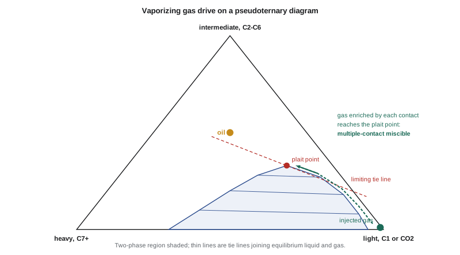
In a vaporizing gas drive, lean gas contacts the oil, vaporizes intermediate components and becomes richer. The enriched gas moves ahead, contacts fresh oil and vaporizes more. If the original oil composition lies on the intermediate-rich side of the limiting tie line that passes through the plait point, the gas at the front eventually becomes miscible with the oil, and the transition zone at the front has no interface. High-pressure lean gas and nitrogen floods work this way in light, intermediate-rich oils. In a condensing gas drive, a rich gas containing intermediates contacts oil and condenses its intermediates into the liquid. The oil near the injector becomes lighter with each contact until it becomes miscible with the injected gas. Rich hydrocarbon gas floods were designed this way in the 1960s and 1970s in Alberta's Devonian reefs.

Later work by Zick in 1986 and by Orr and co-workers showed that most real gas floods, including CO2 floods, are neither purely vaporizing nor purely condensing. With many components, the gas vaporizes some components from the oil while condensing others into it, and miscibility develops in the middle of the transition zone at a crossover tie line rather than at either end. This condensing-vaporizing mechanism explains why rich-gas floods are sometimes effectively miscible at pressures below those predicted by a simple condensing model, and why the minimum miscibility pressure is best computed with a compositional equation-of-state model calibrated to laboratory data rather than read from a ternary diagram.

Minimum miscibility pressure

For a given oil and gas at reservoir temperature, the minimum miscibility pressure (MMP) is the lowest pressure at which the displacement develops multiple-contact miscibility. Below the MMP the displacement is immiscible and recovery drops sharply; above it recovery is high and nearly constant. For CO2, the MMP rises with temperature and with the molecular weight of the heavy fraction of the oil, and falls when the oil is rich in intermediates. Impurities in the CO2 matter too: methane and nitrogen raise the MMP, while hydrogen sulfide and ethane lower it. For hydrocarbon gas the MMP depends strongly on the gas richness, so the operator can choose an enrichment level that gives miscibility at the available pressure.

Correlations give quick estimates for screening. Two that are widely used for pure CO2 in field units are Cronquist's correlation of 1978, which uses temperature, the molecular weight of the C5+ fraction and the mole fraction of methane and nitrogen in the oil, and the Yellig-Metcalfe correlation of 1980, which uses temperature alone:

Both give pressure in psia with temperature in °F. They are valid for typical light oils and moderate temperatures and can differ from each other and from measurements by 10 to 20 percent, so they are never used alone to design a project.

The slim-tube test

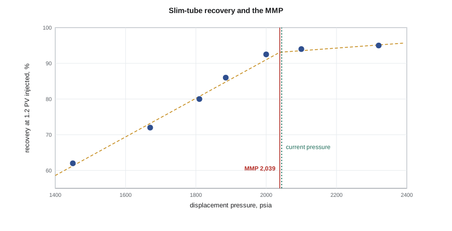
The standard laboratory measurement of MMP is the slim-tube displacement. A long, narrow tube, typically 12 to 24 meters long and a few millimeters in diameter, is packed with sand or glass beads, saturated with the live reservoir oil at reservoir temperature and displaced with the injection gas at constant pressure. The tube is long enough that the transition zone can develop fully and narrow enough that viscous fingering and gravity segregation are suppressed, so the test isolates the phase behavior from sweep. Recovery is measured at 1.2 pore volumes of gas injected. The test is repeated at five or six pressures, and recovery is plotted against pressure. The MMP is taken at the break in the curve, where recovery stops rising steeply; many laboratories also require recovery above 90 percent at the MMP and observe the color and composition of the effluent through a sight glass.

Faster alternatives include the rising bubble apparatus, in which a gas bubble rising through a column of oil is watched for the loss of its interface, and vanishing interfacial tension measurements, in which interfacial tension is extrapolated to zero as pressure rises. They take hours instead of weeks, but they can disagree with slim tubes for condensing-vaporizing systems, so a slim-tube test, an equation-of-state model tuned to swelling and multiple-contact experiments, or both, are standard before a field project.

# CO2 minimum miscibility pressure: two correlations and a slim-tube interpretation.
import math
SI = False     # True: metric units, False: oilfield units
PSI = 6.894757                     # kPa per psi
T_F, mw_c5, vol = 140.0, 190.0, 15.0   # temperature F, C5+ molecular weight, mol% C1 + N2

def cronquist(T, mw, x):           # psia; T in F
    return 15.988 * T ** (0.744206 + 0.0011038 * mw + 0.0015279 * x)

def yellig_metcalfe(T):            # psia; T in F, for 95 to 192 F
    return 1833.7217 + 2.2518055 * T + 0.01800674 * T ** 2 - 103949.93 / T

def show(p_psi):
    return f"{p_psi * PSI:,.0f} kPa" if SI else f"{p_psi:,.0f} psia"

p_res = 2044.0                     # current average pressure, psia
for name, v in (('Cronquist', cronquist(T_F, mw_c5, vol)), ('Yellig-Metcalfe', yellig_metcalfe(T_F))):
    print(f"{name:16s} MMP {show(v):>12s}   margin at {show(p_res)}: {100 * (p_res / v - 1):+5.1f} %")

# slim-tube recovery at 1.2 PV injected
data = [(1450, 62.0), (1670, 72.0), (1810, 80.0), (1885, 86.0), (2000, 92.5), (2100, 94.0), (2320, 95.0)]
def fit(pts):
    n = len(pts); xm = sum(p for p, _ in pts) / n; ym = sum(r for _, r in pts) / n
    b = sum((p - xm) * (r - ym) for p, r in pts) / sum((p - xm) ** 2 for p, _ in pts)
    return ym - b * xm, b
a1, b1 = fit(data[:4]); a2, b2 = fit(data[4:])
mmp = (a2 - a1) / (b1 - b2)
print(f"Slim-tube break in the recovery curve at {show(mmp)}, recovery {a1 + b1 * mmp:.1f} %")
print(f"Pressure for a 10 % margin above the slim-tube MMP: {show(1.10 * mmp)}")

Cronquist        MMP   1,996 psia   margin at 2,044 psia:  +2.4 %
Yellig-Metcalfe  MMP   1,759 psia   margin at 2,044 psia: +16.2 %
Slim-tube break in the recovery curve at 2,039 psia, recovery 93.1 %
Pressure for a 10 % margin above the slim-tube MMP: 2,243 psia

The results bracket the problem nicely. The Yellig-Metcalfe correlation suggests a comfortable margin, Cronquist's correlation a thin one, and the slim-tube test puts the MMP almost exactly at the current average pressure of the pool. In a flood, pressure is highest near the injectors and lowest near the producers, so with no margin a large part of the pattern would run immiscible. Ethan's design will need to raise the average pressure by about ten percent before CO2 injection starts, which the waterflood can do by running a voidage replacement ratio above one for several months.

What miscibility does and does not do

Achieving miscibility guarantees high displacement efficiency in the rock the gas contacts, not high recovery. Recovery still depends on sweep, and miscible gases have very low viscosity and density, so they finger and override. Field CO2 floods in the Permian Basin typically recover an additional 8 to 20 percent of the original oil in place, much less than the 90 percent of the slim tube, because the gas contacts only part of the reservoir and because some oil is shielded from the gas by water. Near-miscible displacements, slightly below the MMP, can still recover much of the oil, because the interfacial tension is very low, so a pool that cannot quite reach the MMP is not necessarily a poor candidate. Lesson 7 turns to how CO2 floods are designed and run to get as much of the slim-tube recovery as possible in the field.

Swelling and multiple-contact tests

Besides the slim tube, a PVT laboratory supporting a gas project runs swelling tests, in which known amounts of gas are added to the live oil and the saturation pressure and oil volume are measured at each step, and multiple-contact experiments, in which gas and oil are mixed, separated and contacted again with fresh fluid to mimic the forward or backward contacts in the reservoir. These data are used to tune the equation of state that the compositional simulator will use. Without such tuning, a simulator can predict an MMP several megapascals away from the true value, and every forecast built on it inherits the error.