Mobility ratio and volumetric sweep

The second half of the recovery product is sweep. Lena hands Ethan the pilot simulation from two years ago and asks a pointed question: “The model said the thief layer took three quarters of the water. How much of the pool has the water actually touched, and what would a different injectant do to that number?” Answering it requires two ideas that underlie every injection project: the mobility ratio, which controls how evenly a displacing fluid advances, and reservoir heterogeneity, which controls where it goes.

Mobility and mobility ratio

The mobility of a fluid in a rock is its effective permeability divided by its viscosity, λ = k k_r / μ. It measures how easily the fluid flows under a given pressure gradient. When one fluid displaces another, the outcome depends on their relative mobility, expressed by the mobility ratio:

The most common convention, used by Craig and by Dykstra and Parsons, evaluates the water relative permeability at the residual oil saturation behind the front and the oil relative permeability at the connate water saturation ahead of it. This is the endpoint mobility ratio. A mobility ratio of one or less is called favorable: the displacing fluid is no more mobile than the oil, the front stays stable and the displacing fluid advances like a piston. A mobility ratio above one is unfavorable: any small bulge in the front advances faster than its surroundings, grows into a finger, and the displacing fluid breaks through early. Some authors use a shock-front mobility ratio evaluated with the average saturation behind the front from the Buckley-Leverett solution, which is a better predictor of frontal stability; for a favorable flood the two definitions give similar values.

For the Mission Canyon pool, with endpoint relative permeabilities of 0.30 for water and 0.80 for oil, the waterflood mobility ratio is about 0.7. That is favorable, which is why the pilot responded so well. Carbon dioxide, with a reservoir viscosity near 0.06 cp, has a mobility ratio of six or more against the same oil. Gas floods are almost always unfavorable, and much of the art of gas EOR in Lessons 7 and 8 is controlling that mobility. Heavy oil waterfloods are worse still: a 1,000 cp oil gives a waterflood mobility ratio in the hundreds, which is the reason polymer flooding was developed.

Areal sweep

Areal sweep efficiency is the fraction of the pattern area contacted by the displacing fluid. Even with M = 1, the flow lines in a pattern converge on the producer, so the injected fluid arrives first along the shortest streamline and leaves the corners of the pattern unswept. Physical scaled models built in the 1950s and 1960s, with potentiometric and X-ray shadowgraph techniques, measured areal sweep for the common patterns as a function of mobility ratio. Craig's monograph collects them. For a five-spot, areal sweep at breakthrough is about 0.70 at M = 1, rises toward one for very favorable mobility ratios, and falls toward 0.5 at M = 10.

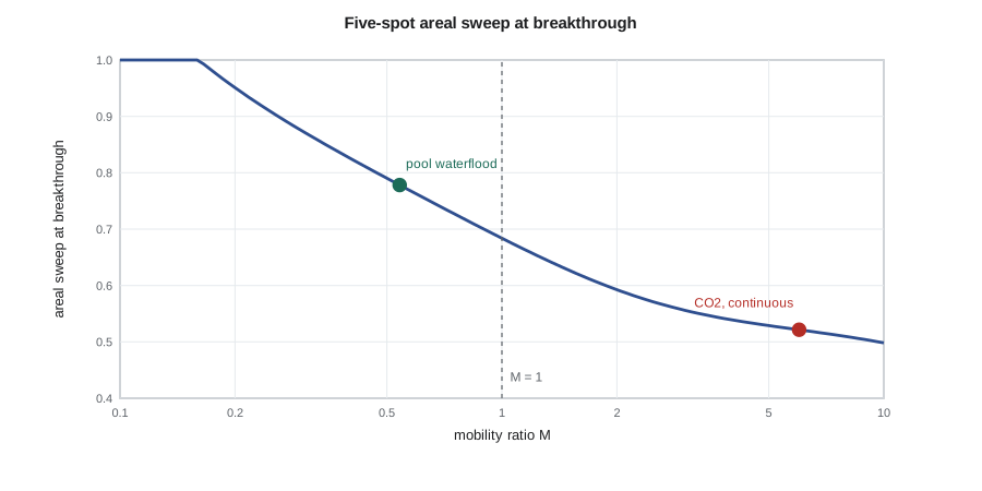
Areal sweep keeps rising after breakthrough as more fluid passes through the pattern, and the scaled-model data also give sweep as a function of the displaceable pore volumes injected. A useful fit to Craig's five-spot data at breakthrough, often quoted in textbooks, is:

The fit is valid for mobility ratios from about 0.1 to 10. Like all scaled-model results, it assumes a homogeneous, isotropic layer; directional permeability, natural fractures and faults change areal sweep in ways only a geological model can capture.

Vertical sweep and heterogeneity

Real reservoirs are layered. In the Mission Canyon pool the permeability varies from a few millidarcies to more than a hundred within a few meters of section, and the layers are separated by thin shales or tight streaks that limit vertical flow. Injected water enters each layer roughly in proportion to its flow capacity, kh, so it races through the best layers and lags in the poor ones. Vertical sweep, or invasion efficiency, is the fraction of the vertical section contacted at a given time.

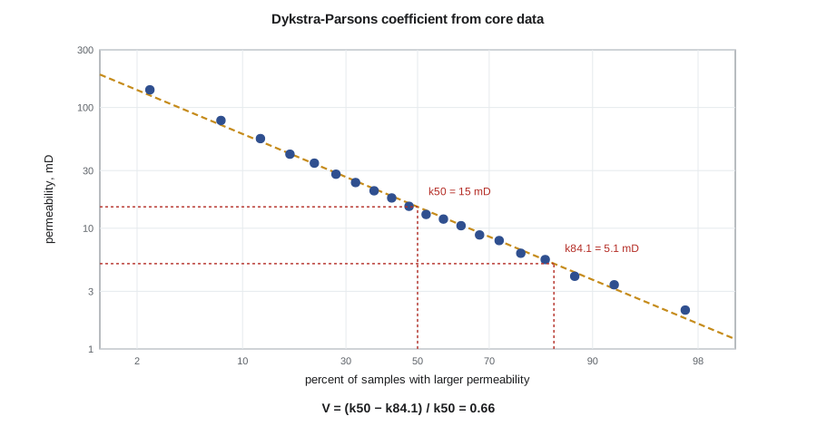
In 1950 Dykstra and Parsons proposed a measure of layered heterogeneity and a method to compute the vertical coverage of a waterflood in non-communicating layers. Permeability in many reservoirs is approximately log-normally distributed. If the core permeabilities are plotted on a log-probability scale, they fall close to a straight line. The Dykstra-Parsons coefficient is defined from that line as:

where k_50 is the median permeability and k_84.1 the permeability exceeded by 84.1 percent of the samples, one standard deviation below the median of the logarithm. V is zero for a uniform reservoir and approaches one for an extremely heterogeneous one. Most sandstone reservoirs fall between 0.5 and 0.9; values above about 0.8 make waterflooding difficult and conformance control valuable.

In the Dykstra-Parsons layer model, each layer is treated as a separate one-dimensional piston displacement with the same pressure drop. A high-permeability layer breaks through first. At that moment the front in a tighter layer with permeability ratio r = k_i / k_j to the broken-through layer has advanced a fraction x of the distance, where for M = 1 simply x = r, and for other mobility ratios:

The vertical coverage is the average of the front positions over all layers. The method assumes no crossflow between layers, piston-like displacement and equal porosity and saturation in each layer, so it is a screening tool. A simulator is needed when layers communicate, because crossflow driven by viscous and gravity forces can either help, by letting water enter the tight layers from the side, or hurt, by letting it slump into the bottom of a layer.

# Mobility ratio, five-spot areal sweep and Dykstra-Parsons layer coverage.
import math, statistics
SI = False     # True: metric units, False: oilfield units

mu_o = 0.72 if SI else 0.95          # oil viscosity, mPa.s or cp
kro, krw, krg = 0.80, 0.30, 0.40      # endpoint relative permeabilities
cases = {'water': (krw, 0.50), 'polymer, 3 cp': (krw * 0.6, 3.0), 'CO2': (krg, 0.06)}

def ea_bt(M):
    """Areal sweep of a five-spot at breakthrough (fit to Craig's data)."""
    return 0.54602036 + 0.03170817 / M + 0.30222997 / math.exp(M) - 0.00509693 * M

print(f"Oil viscosity {mu_o} " + ("mPa·s" if SI else "cp"))
for name, (kr, mu) in cases.items():
    M = (kr / mu) / (kro / mu_o)
    print(f"  {name:15s} M = {M:6.2f}   five-spot sweep at breakthrough {min(ea_bt(M), 1.0):.2f}")

# Dykstra-Parsons coefficient from 20 core plugs (mD)
k = [2.1, 3.4, 4.0, 5.5, 6.2, 7.9, 8.8, 10.5, 11.9, 13.0,
     15.2, 17.8, 20.4, 23.9, 28.0, 34.6, 41.0, 55.2, 78.0, 140.0]
lk = [math.log(x) for x in k]
mu_l, sd_l = statistics.mean(lk), statistics.stdev(lk)
k50, k84 = math.exp(mu_l), math.exp(mu_l - sd_l)
V = (k50 - k84) / k50
print(f"k50 = {k50:.1f} mD, k84.1 = {k84:.1f} mD, V = {V:.2f}")

def coverage(perms, M):
    """Vertical coverage when each layer in turn breaks through (equal thickness and porosity)."""
    ks = sorted(perms, reverse=True); n = len(ks); out = []
    for j in range(n):
        tot = j + 1
        for kk in ks[j + 1:]:
            r = kk / ks[j]
            x = r if abs(M - 1) < 1e-9 else (M - math.sqrt(M * M + r * (1 - M * M))) / (M - 1)
            tot += x
        out.append(tot / n)
    return out

for M in (0.5, 1.0, 5.0):
    c = coverage(k, M)
    print(f"  M = {M:3.1f}: coverage {c[0]:.2f} at first breakthrough, {c[4]:.2f} after five layers")

Oil viscosity 0.95 cp
  water           M =   0.71   five-spot sweep at breakthrough 0.74
  polymer, 3 cp   M =   0.07   five-spot sweep at breakthrough 1.00
  CO2             M =   7.92   five-spot sweep at breakthrough 0.51
k50 = 15.0 mD, k84.1 = 5.1 mD, V = 0.66
  M = 0.5: coverage 0.23 at first breakthrough, 0.56 after five layers
  M = 1.0: coverage 0.19 at first breakthrough, 0.51 after five layers
  M = 5.0: coverage 0.14 at first breakthrough, 0.43 after five layers

The output tells a consistent story. Water against the light pool oil is favorable, so the areal sweep at breakthrough is high. Carbon dioxide is strongly unfavorable and the areal sweep at breakthrough falls to about half. The core plugs give V = 0.66, a moderately heterogeneous reservoir, and the layer calculation shows that only about a fifth of the section is contacted when the best layer breaks through. Coverage improves as more layers break through, and it is always better for a lower mobility ratio, which is why polymer can improve vertical sweep even in a light oil flood when the layers are strongly contrasted.

Sweep in gas floods: gravity and viscous fingering

Two further effects dominate sweep in gas floods. The first is gravity override. Injected gas is much less dense than oil and water, so it rises to the top of the formation and flows along it, leaving the lower part unswept; water injected after it does the reverse and underruns the oil. The balance between viscous and gravity forces is measured by a viscous-to-gravity ratio, and thick, vertically permeable reservoirs suffer most. The second is viscous fingering at the small scale: in an unfavorable miscible displacement the front breaks into fingers that a coarse simulation grid cannot resolve, so simulators use empirical mixing parameters such as the Todd-Longstaff model to represent their average effect.

Both effects explain why gas floods are rarely run as continuous gas injection. Alternating slugs of water and gas, the WAG process of Lesson 7, reduce the effective mobility of the gas, spread the injectant through more of the section and make use of the water's tendency to sweep the lower layers. Foams, polymer-thickened water and conformance gels are further tools. In each case the engineer is working on E_V, the volumetric sweep, while relying on the miscible gas or surfactant for E_D.

For Ethan, the sweep analysis sharpens the choice. The Mission Canyon pool waterflood already has a favorable mobility ratio, so its weakness is vertical sweep in a layered sand. Any tertiary process will have to deal with the same thief layer, and a gas process will make it worse unless the mobility is controlled.

Field engineers often combine the two sweep factors into a single quick check. Multiplying the areal sweep from the scaled-model data by the Dykstra-Parsons coverage for the same mobility ratio gives a volumetric sweep that is usually within about ten percent of a simulation result for the same pattern, provided the layers do not communicate strongly. Ethan's check for the pilot pattern gives 0.47 against the simulator's 0.46.