Carbonates and fractured reservoirs

Below the Bakken, the Tamarack 8-27 pilot well was deepened through the Three Forks and into the Mission Canyon Formation, a carbonate that Prairie Crest Energy Inc. produces from in the Mission Canyon pool and also uses for water disposal. Mei Lin asked for a log evaluation of it before designing acid treatments. 'Carbonates break most of the rules you learned on sandstones,' Imogen warns Ethan. 'The porosity can be in vugs, molds or fractures as well as between grains, the cementation exponent changes with pore type, and two rocks with the same porosity can differ in permeability by a thousand times.'

This lesson covers the features that make carbonate and fractured reservoirs hard to evaluate: complex lithology, varied pore types, the secondary porosity index, the effect of pore type on the cementation exponent, fracture detection with logs and borehole images, and how all of these feed permeability and flow predictions.

Carbonate lithology

Carbonate reservoirs are mostly limestone (calcite) and dolomite, often mixed, with anhydrite, gypsum, chert, clay and quartz. Dolomite forms when magnesium-rich fluids alter limestone; the process can create porosity, because dolomite crystals are smaller than the calcite they replace, or destroy it when dolomite cement fills pores. Anhydrite commonly fills pores in evaporite-associated carbonates and has a very high density and low porosity.

With several minerals present, no single porosity tool gives porosity directly, because each mineral has its own matrix values. The neutron-density crossplot of lesson 6 is the standard first step: limestone and dolomite lines separate clearly, and points between them indicate a mixture. The photoelectric factor separates calcite (about 5) from dolomite (about 3) and flags anhydrite by its high density with a Pe near 5. With three or more minerals, petrophysicists solve multi-mineral models that combine density, neutron, Pe, sonic and sometimes spectral gamma ray simultaneously, finding the mineral volumes and porosity that best match all the logs.

Pore types in carbonates

Carbonate pores are classified by their geometry and origin. Interparticle pores lie between grains, like sandstone pores, and are common in grainstones and oolites. Intercrystalline pores lie between dolomite crystals in sucrosic dolomites, often with good connectivity. Moldic pores form where grains such as shells or ooids dissolve, leaving holes that may be poorly connected to each other. Vugs are larger irregular cavities from dissolution. Fractures are planar cracks that can be very permeable even when they add little porosity. Classification schemes by Choquette and Pray, and by Lucia, are used to describe them and to relate them to permeability.

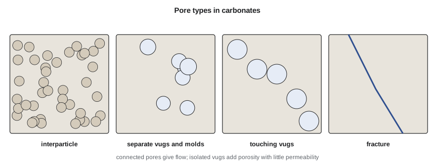
Lucia's work showed that separate-vug porosity, in vugs connected only through the matrix, adds to porosity but little to permeability, while touching-vug porosity, including fractures and connected large vugs, can dominate flow. Interparticle porosity controls permeability in most carbonates, and its relation to permeability depends on particle size, which can be grouped into rock-fabric classes. This framework is central to building permeability models for carbonate fields.

The secondary porosity index

As lesson 6 explained, the sonic tool sees mainly the porosity in the continuous grain framework and largely misses isolated vugs and molds. Neutron and density respond to all the pore volume. The difference between total porosity from neutron-density and sonic porosity is therefore an estimate of secondary porosity.

# Secondary porosity in a carbonate, and how the cementation exponent changes the saturation
SI = False  
phi_t = 0.115                         # neutron-density total porosity
if SI: dt, dtma, dtf = 190.0, 156.0, 620.0
else:  dt, dtma, dtf = 57.8, 47.5, 189.0
phi_s = (dt - dtma) / (dtf - dtma)    # sonic sees mainly intergranular/matrix porosity
spi = phi_t - phi_s
print(f"total porosity {phi_t:.3f}, sonic porosity {phi_s:.3f}, secondary porosity index {spi:.3f}")
rw, rt, a, n = 0.03, 12.0, 1.0, 2.0
for label, m in (("intergranular, m = 2.0", 2.0), ("vuggy, m = 2.4", 2.4), ("fractured, m = 1.6", 1.6)):
    sw = (a * rw / (phi_t ** m * rt)) ** (1 / n)
    print(f"{label:24s} Sw = {sw:.2f}")

total porosity 0.115, sonic porosity 0.073, secondary porosity index 0.042
intergranular, m = 2.0   Sw = 0.43
vuggy, m = 2.4           Sw = 0.67
fractured, m = 1.6       Sw = 0.28

In the Mission Canyon interval of the Tamarack 8-27 pilot well, neutron-density porosity is 11.5 percent and Wyllie sonic porosity is 7.3 percent, giving a secondary porosity index of about 4 percent. Core plugs confirm moldic and vuggy porosity from dissolved fossil fragments. The index flags where the porosity is likely to be poorly connected, which matters for both saturation and permeability.

Pore type and the cementation exponent

The cementation exponent m in Archie's equation reflects how tortuous the current path is. In rocks with isolated vugs or molds, current must travel through the matrix around the vugs, so the vugs add porosity but little conduction; the effective m rises above 2, often to 2.3 to 3 or more. In fractured rocks the fractures provide straight conductive paths, and m falls toward 1.3 to 1.6. Using m = 2 in these rocks gives systematic errors.

The program shows the size of the effect. For the same porosity, Rt and Rw, saturation is 43 percent with m = 2.0, 67 percent with m = 2.4 and 28 percent with m = 1.6. Choosing m for a carbonate is therefore not a minor detail; it can decide whether an interval is pay. Several methods estimate m from logs, including relating it to the secondary porosity index or the vug fraction, and dual-porosity models treat matrix and fractures with separate exponents. Core measurements of formation factor on plugs that include the vugs remain the best guide, though plugs often under-represent large vugs and fractures.

Detecting fractures

Natural fractures matter because they can carry most of the flow in a tight reservoir, or they can short-circuit a waterflood or a hydraulic fracture. Logs detect them in several ways, none perfect on its own.

Borehole images are the most direct. Micro-resistivity imagers press many small electrodes against the borehole wall and build a picture of resistivity around the hole; ultrasonic imagers measure the amplitude and travel time of sound reflected from the wall. Open fractures filled with conductive mud appear as dark sinusoidal traces on the unrolled image, because a plane cutting a cylinder plots as a sine wave. The amplitude and position of the sine wave give the fracture's dip and dip direction. Images also show bedding, stylolites, vugs and drilling-induced fractures and breakouts that reveal the stress direction.

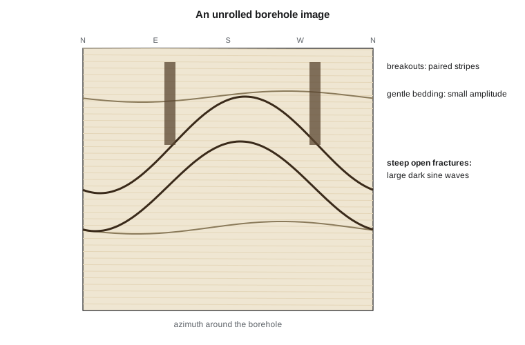
Other indications include caliper enlargements where fractured rock has broken out; sonic waveform changes, because fractures attenuate shear and Stoneley waves, and Stoneley-wave reflections that mark open fractures; resistivity differences between shallow and deep curves where conductive mud has invaded fractures; and mud losses during drilling. Drilling-induced fractures, which form in the borehole wall from drilling stresses, must be distinguished from natural fractures on images, since they do not extend into the formation.

Fracture porosity and permeability

Fractures usually add less than one percent porosity but can add enormous permeability. Parallel-plate flow theory shows that the flow through a smooth fracture scales with the cube of its aperture, so a fracture just a fraction of a millimeter wide can carry more flow than meters of tight matrix. Fracture apertures are estimated from image resistivity anomalies or from core, but both are uncertain, and the effective aperture at reservoir stress may be much smaller than that seen in the borehole wall. Well tests and production data usually give the most reliable measure of fracture contribution.

For the Mission Canyon wells, the images in the Tamarack 8-27 pilot well show a set of open fractures striking roughly northeast, parallel to the maximum horizontal stress shown by drilling-induced fractures. Mei Lin will use that direction in designing acid jobs, and Tom Ashworth notes that the same stress direction controls hydraulic fracture orientation in the Bakken horizontals.

Evaluating carbonates in practice

A practical carbonate workflow solves for lithology and porosity with a multi-mineral model, estimates secondary porosity, chooses m and n by pore type with core support, checks fracture indications on images and other logs, and then predicts permeability by rock-fabric class rather than by a single porosity-permeability line. Nuclear magnetic resonance, covered in lesson 10, adds pore-size information that helps separate small pores from vugs. Throughout, the interpreter should expect larger uncertainty than in clean sandstones and report it.

Rock-fabric classes and permeability

In sandstones a single porosity-permeability line from core often works across a reservoir. In carbonates it rarely does, because rocks with the same porosity can have very different pore-throat sizes. Lucia grouped interparticle porosity by the size of the particles or crystals: grainstones and large crystalline dolomites, with particles larger than about 100 micrometers, have the largest pores and highest permeability for a given porosity; grain-dominated packstones and medium crystalline dolomites form a middle class; and mud-dominated fabrics and fine crystalline dolomites have the smallest pores and lowest permeability. Each class has its own porosity-permeability trend and its own capillary pressure behavior. Identifying the class from core descriptions, and then predicting it from logs where core is absent, is the key step in carbonate permeability modeling.

Other methods use pore-throat size directly. Mercury injection capillary pressure gives the pore-throat size distribution of a plug, and the throat radius at a particular mercury saturation, such as the r35 of the Winland method, correlates well with permeability across rock types. NMR T2 distributions (lesson 10) give a continuous pore-size indication in the well that can be tied to these classes.

Dolomite and reservoir quality

The Mission Canyon in this part of the Tamarack Lake field shows how diagenesis controls carbonate quality. Where the original limestone was dolomitized, crystal sizes grew and intercrystalline porosity developed, giving the best reservoir. Where later anhydrite filled the pores, porosity was lost. On the logs, the best intervals show Pe near 3, density porosity of 10 to 15 percent on a dolomite matrix and low gamma ray; the tight anhydritic intervals show high density, Pe near 5 and almost no porosity. Mapping these facies between wells guides where the Mission Canyon pool can be developed and where water can be injected without returning to producing zones.

Fractures in tight rock

In very tight rocks such as many shales and tight carbonates, natural fractures can be the difference between a commercial and an uncommercial well, but they can also be closed or mineralized and contribute nothing. Images show whether fractures are open (dark, conductive in water-based mud) or filled with calcite or other cement (bright, resistive). Core shows the same and allows the fracture fill to be identified. Orientation matters too: fractures parallel to the maximum horizontal stress are more likely to stay open under reservoir stress than fractures at a high angle to it. These observations feed the completion design, because hydraulic fractures interact with natural fractures and can either connect them usefully or be diverted by them.

Images beyond fractures

Borehole images are used for much more than fractures. Bedding dips from images give the structural dip at the well and, in cross-bedded sands, the direction in which ancient currents flowed, which helps predict how sand bodies are oriented between wells. Stylolites, irregular dissolution surfaces common in carbonates, show as jagged dark traces and can act as barriers to vertical flow. Vugs show as dark or bright spots depending on their fill, and image-based porosity analysis can estimate the vug fraction directly, an independent check on the secondary porosity index. Breakouts and drilling-induced fractures give the stress directions that completion engineers need.