Tight and shale reservoirs

The Bakken is the reservoir Prairie Crest Energy Inc. already produces, and it is a tight-oil play: the middle member has porosities of 4 to 8 percent and matrix permeabilities in the microdarcy range, sandwiched between upper and lower shales that are among the richest source rocks in North America. Lena has asked Ethan to reconcile the core data with the production data. He soon finds that almost every method in the earlier lessons needs to be changed. 'Tight rock breaks the rules we learned in conventional sandstone,' she tells him. 'Permeability in micro- and nanodarcies, pores you need an electron microscope to see, gas that slides along pore walls, and porosity that depends on how you dry the sample. The rock physics is the same, but the numbers are so extreme that the methods have to change.'

What makes a reservoir tight

There is no single definition, but tight reservoirs are generally those with matrix permeability below about 0.1 mD, too low to produce at economic rates without hydraulic fracturing or other stimulation. Tight gas sandstones, tight oil siltstones and carbonates, and shales form a continuum. In shale, the source rock is itself the reservoir: oil and gas generated from organic matter remain in the rock's tiny pores instead of migrating out. In tight-oil plays such as the middle Bakken or the Montney siltstone, the reservoir is a low-permeability rock next to or interbedded with a source rock. Production from these resources transformed North American oil and gas output after about 2008, when horizontal drilling and multistage hydraulic fracturing were combined at scale.

Pores in shale

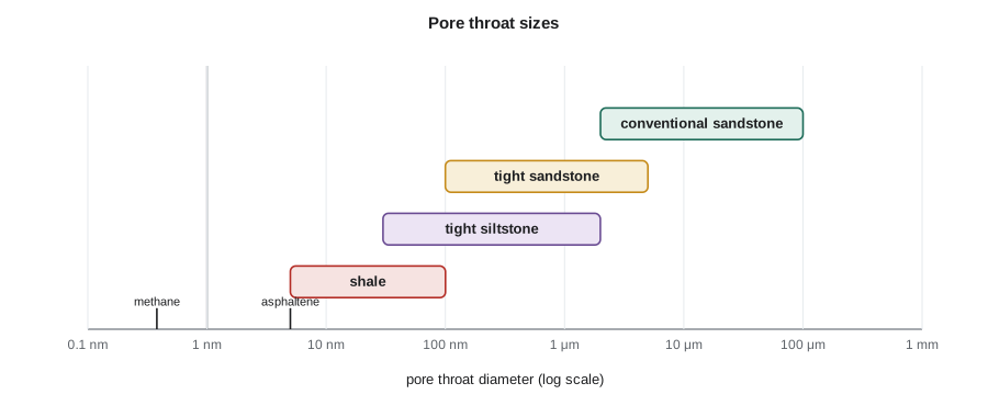
Scanning electron microscope images of ion-milled shale surfaces show several kinds of pores. Interparticle pores lie between mineral grains, usually clay, quartz silt and carbonate. Intraparticle pores lie inside grains, such as within fossil fragments or clay aggregates. Organic pores, often only tens of nanometers across, form inside kerogen and solid bitumen as hydrocarbons are generated and expelled, and they can account for much of the porosity in mature gas shales. Organic pores tend to be oil-wet or hydrocarbon-wet, while mineral pores are more often water-wet, giving shales a mixed wettability at a very small scale.

Pore size matters for more than permeability. In pores of a few nanometers, a significant fraction of the gas is adsorbed onto organic and clay surfaces instead of being free in the pore space. Adsorbed gas, described by the Langmuir isotherm, is released only as pressure falls, so it contributes to production late in a well's life. In shale gas resource estimates, adsorbed gas can be 20 to 50 percent of the total in some plays.

In the Langmuir equation, Va is the adsorbed gas volume per unit mass of rock, VL is the Langmuir volume, the maximum adsorbed at infinite pressure, and pL is the Langmuir pressure, at which half of VL is adsorbed. Both are measured on crushed samples in the laboratory.

Measuring porosity in tight rock

Plug porosity measurements struggle in tight rock because helium takes a very long time to reach all the pores and because microcracks created when the core is unloaded add porosity that does not exist underground. The Gas Research Institute method, developed for shale in the 1990s, crushes the sample to particles about 0.5 to 0.85 mm across, so helium has a short distance to travel. Crushed-rock porosity is usually reported together with saturations from Dean-Stark extraction of the crushed material. Crushing also removes microcracks from the measurement, although results still vary between laboratories with crushing size and drying temperature.

Drying conditions control which water is counted as pore water. Drying at 110 °C removes clay-bound water and gives something close to total porosity; humidity-controlled drying at about 60 °C leaves clay-bound water in place and gives a value nearer effective porosity. Nuclear magnetic resonance, in the laboratory and as a logging tool, can partition porosity by pore size and fluid type and is widely used in shale evaluation. The important point for Ethan is that porosity numbers from different laboratories and methods are not directly comparable unless the procedures are the same.

Measuring permeability in tight rock

Steady-state gas flow through a nanodarcy plug would take far too long to stabilize. The pulse-decay method instead applies a small pressure pulse to one end of a confined plug and records how the pressure difference decays as gas moves through; permeability is found from the decay rate. It works down to about a nanodarcy. The crushed-rock or GRI permeability method measures pressure decay into crushed particles and reaches even lower values, but it measures the matrix without microfractures or bedding laminae, and results from different methods on the same rock can differ by an order of magnitude or more. Engineers therefore treat tight-rock permeability as uncertain and calibrate it against production data.

Stress sensitivity is much stronger in tight rock than in conventional sandstone. Sheet-like pores and microcracks close as effective stress rises, so permeability measured at low confining stress can be several times higher than at reservoir stress. Measurements should always be made at representative effective stress.

Gas slip and Knudsen flow

Lesson 3 introduced gas slip and the Klinkenberg correction. In shale the effect becomes dominant. The Knudsen number, Kn, compares the mean free path of gas molecules, the average distance between collisions, to the pore diameter. When Kn is below about 0.001, gas behaves as a continuum and Darcy's law holds. Between 0.001 and 0.1, slip flow occurs and Klinkenberg's correction applies. Above 0.1, transition and free-molecular flow occur, in which molecules collide with walls more than with each other. As a shale gas reservoir is depleted, falling pressure lengthens the mean free path and raises Kn, so the apparent permeability of the matrix actually increases.

# Why tight rock needs fractures: pressure diffusion time and gas slip in nanometer pores
import math
phi, mu, ct = 0.06, 0.5e-3, 3.0e-9          # porosity, oil viscosity Pa.s, total compressibility 1/Pa
print("permeability      time to diffuse 10 m     time to diffuse 100 m")
for k_md in (100, 1, 0.01, 0.0001):
    k = k_md * 0.9869e-15
    D = k / (phi * mu * ct)                   # hydraulic diffusivity, m2/s
    t10, t100 = 10 ** 2 / D, 100 ** 2 / D
    def fmt(t):
        d = t / 86400
        if d < 1: return f"{t / 60:10.1f} minutes" if t < 3600 else f"{t / 3600:10.1f} hours"
        return f"{d:10.1f} days" if d < 365 else f"{d / 365:10.1f} years"
    print(f"{k_md:10.4f} mD {fmt(t10)} {fmt(t100)}")

# Knudsen number: mean free path of methane over pore diameter
kB, T, d_mol = 1.380649e-23, 360.0, 0.38e-9
for p_mpa in (30, 10, 2):
    lam = kB * T / (math.sqrt(2) * math.pi * d_mol ** 2 * p_mpa * 1e6)
    for d_nm in (1000, 50, 10):
        kn = lam / (d_nm * 1e-9)
        regime = "continuum (Darcy)" if kn < 0.001 else ("slip flow" if kn < 0.1 else "transition")
        print(f"p {p_mpa:2d} MPa, pore {d_nm:4d} nm: Kn = {kn:.4f} -> {regime}")

permeability      time to diffuse 10 m     time to diffuse 100 m
  100.0000 mD        1.5 minutes        2.5 hours
    1.0000 mD        2.5 hours       10.6 days
    0.0100 mD       10.6 days        2.9 years
    0.0001 mD        2.9 years      289.2 years
p 30 MPa, pore 1000 nm: Kn = 0.0003 -> continuum (Darcy)
p 30 MPa, pore   50 nm: Kn = 0.0052 -> slip flow
p 30 MPa, pore   10 nm: Kn = 0.0258 -> slip flow
p 10 MPa, pore 1000 nm: Kn = 0.0008 -> continuum (Darcy)
p 10 MPa, pore   50 nm: Kn = 0.0155 -> slip flow
p 10 MPa, pore   10 nm: Kn = 0.0775 -> slip flow
p  2 MPa, pore 1000 nm: Kn = 0.0039 -> slip flow
p  2 MPa, pore   50 nm: Kn = 0.0775 -> slip flow
p  2 MPa, pore   10 nm: Kn = 0.3874 -> transition

The first half of the program explains why tight rock must be fractured. Pressure disturbances spread by diffusion, and the time to travel a distance L scales with φμctL²/k. In 100 mD rock, pressure diffuses 100 m in a few hours. In 0.0001 mD rock, the same distance would take nearly three centuries. Production from tight rock comes only from the matrix within a few meters of fracture surfaces. Hydraulic fracturing creates a large surface area of contact so that the short distances add up to economic volumes. The second half shows Knudsen numbers for methane: in 10-nanometer pores at low pressure, flow enters the transition regime where Darcy's law no longer applies.

Saturation and fluids in tight rock

Archie's law, from lesson 5, is hard to apply in shale. Clay conductivity, pyrite and conductive mature organic matter lower resistivity, and the cementation and saturation exponents are uncertain. Water saturation is often estimated from Dean-Stark analysis of crushed preserved core and from NMR, then compared with log models calibrated to those core data. Many productive shales have water saturations below their irreducible values in conventional terms, a condition called subirreducible saturation, possibly because hydrocarbon generation consumed or expelled water. These rocks can imbibe water strongly, which affects how much fracturing fluid returns to the surface.

Fluid behavior can also change. In pores only a few nanometers across, the fluid near the walls behaves differently from bulk fluid, and laboratory and theoretical studies suggest that confinement can shift bubble points and reduce viscosities. Total organic carbon, thermal maturity and the type of kerogen, covered in PET-210, control whether a shale produces mainly oil, condensate or dry gas.

Key properties for evaluating a tight play

Evaluation of tight plays relies on a broader set of properties than conventional reservoirs. Reservoir quality depends on porosity, permeability, saturation, total organic carbon, maturity and thickness. Completion quality depends on mineralogy, brittleness, stress and natural fractures, which control how well the rock fractures; lesson 11 covers the mechanical side. Sweet spots, where both are favorable, can produce several times more than average areas, so mapping them across a play is worth a great deal.

For the Bakken, Ethan builds a table of the properties that core and logs can provide and the methods needed: crushed-rock porosity and saturation, pulse-decay permeability at stress, Rock-Eval and TOC on the shales, mineralogy by X-ray diffraction, mechanical properties and NMR. Lena reminds him that, in the end, the best test of tight-rock properties is the production from wells, and the company has hundreds of them to learn from.