
MEC-499 · Lesson 6 of 12 · 24 min
Detailed design and analysis
Detailed design turns the embodied layout into something that can be built and trusted: every part dimensioned, every material and fastener specified, and every load path checked. Analysis is how the team gains confidence that the design will meet its requirements before steel is cut. In a capstone the temptation is to analyze whatever the team knows how to analyze, in as much detail as the software allows. The better approach is to ask which requirements are at risk, analyze those first with the simplest method that answers the question, and reserve detailed tools such as finite elements for the places where simple methods are not enough.
Kwame drew up an analysis plan in week 7 listing each requirement, the risk to it, the analysis that would address it and the method. This lesson follows the four analyzes that mattered most: the hydraulics, the frame, fatigue in transport and vibration isolation.
The analysis plan
| Requirement at risk | Question | Method | Reference course |
|---|---|---|---|
| R-01 flow, R-03 deep lift | Where does the pump operate, and will it cavitate? | pump and system curves, NPSH | MEC-370 Fluid Mechanics II |
| R-06 run time | How much fuel at the rated point? | power from the operating point, engine fuel map | MEC-330 Thermodynamics II |
| R-05 mass, R-12 transport | Is the frame strong enough, and is it heavier than needed? | beam bending, then finite elements at the lifting points | MEC-450 Finite Element Analysis |
| R-12 transport | Will welds crack under road vibration over 10 years? | weld fatigue with a detail category and Miner's rule | MEC-360 Machine Design |
| R-07 noise, frame life | Will engine vibration reach the frame and canopy? | isolator transmissibility | MEC-380 Mechanical Vibrations |
Hydraulics: the operating point
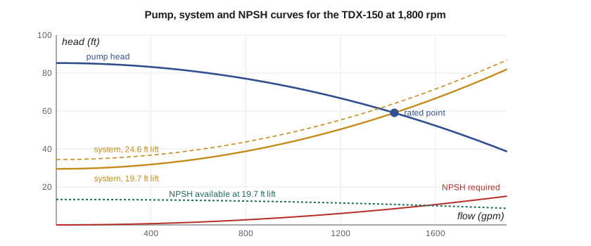
A centrifugal pump does not deliver a fixed flow. It delivers whatever flow makes the head it produces equal the head the system demands. The pump's head falls as flow rises; the system's demand rises with flow because friction grows with velocity squared. The operating point is where the two curves cross. For a skid like this, the system curve has a static part, the height from the water surface to the discharge point, and a dynamic part from friction in the suction hose, the pump fittings and the discharge hose.
Tidewater's test data for its 150 mm wet end at 1,800 rpm fit a shutoff head of 26 m falling to 18 m at 90 L/s, with best efficiency of 68 percent at that point. Kwame fitted simple quadratics to both curves, which is accurate enough near the operating point:
Here z_s is the suction lift and z_d the 3 m rise from the pump to the discharge. The loss coefficient k_s came from the friction of 60 m of 150 mm lay-flat hose, a foot strainer and the suction hose, calculated with the methods of the fluid mechanics courses. Setting the two heads equal gives the flow directly.
Hydraulics: suction lift and NPSH
A pump above the water lifts it by lowering the pressure at its inlet below atmospheric pressure. The pressure cannot fall below the water's vapor pressure without the water boiling in the impeller eye, which is cavitation: noisy, damaging and the end of the rated flow. The margin is measured by net positive suction head. The head available at the pump inlet is
and it must exceed the head the pump requires, NPSHr, which the manufacturer measures as the point at which head drops by 3 percent. Standards and good practice call for a margin above NPSHr, commonly expressed as a ratio, because NPSHr itself marks the onset of measurable cavitation, not its absence. The program finds the operating point at three suction lifts and checks the NPSH margin at each.
# TDX-150 hydraulics: operating point, NPSH margin, shaft power and fuel for 24 h
import math
rho, g = 1000.0, 9.81
H0, kp = 26.0, 8.0 / 90**2        # pump at 1,800 rpm: H = H0 - kp Q^2 (Q in L/s, H in m)
def eff(Q): return 0.68 - 0.68 * ((Q - 90) / 90) ** 2     # best efficiency 68 % at 90 L/s

def op_point(static, ks):
    Q = math.sqrt((H0 - static) / (kp + ks)); return Q, H0 - kp * Q * Q

ks = 9.0 / 90**2                  # 60 m of 150 mm lay-flat hose plus fittings
for lift in (4.0, 6.0, 7.5):
    static = lift + 3.0               # suction lift plus 3 m rise to the discharge point
    Q, H = op_point(static, ks)
    P = rho * g * Q / 1000 * H / eff(Q) / 1000
    hs = 0.8 * (Q / 90) ** 2          # suction hose, strainer and foot-valve losses
    npsha = 101.3e3 / (rho * g) - lift - hs - 2.34e3 / (rho * g)
    npshr = 2.6 * (Q / 90) ** 2
    print(f"lift {lift:3.1f} m: Q {Q:5.1f} L/s, H {H:4.1f} m, shaft {P:4.1f} kW, "
          f"NPSHa {npsha:4.2f} m vs NPSHr {npshr:4.2f} m (ratio {npsha / npshr:4.2f})")

# Fuel for 24 h at the rated point (6 m lift) with priming system and alternator loads
Q, H = op_point(9.0, ks)
P_engine = rho * g * Q / 1000 * H / eff(Q) / 1000 + 0.9
bsfc = 0.235                          # kg/kWh at about 75 % load, typical small industrial diesel
fuel_L = P_engine * bsfc / 0.84 * 24
print(f"Engine load {P_engine:.1f} kW, fuel {fuel_L / 24:.2f} L/h, {fuel_L:.0f} L per 24 h")
print(f"Usable 180 L of a 200 L tank lasts {180 / (fuel_L / 24):.1f} h")lift 4.0 m: Q 95.1 L/s, H 17.1 m, shaft 23.5 kW, NPSHa 5.19 m vs NPSHr 2.91 m (ratio 1.79) lift 6.0 m: Q 90.0 L/s, H 18.0 m, shaft 23.4 kW, NPSHa 3.29 m vs NPSHr 2.60 m (ratio 1.26) lift 7.5 m: Q 85.9 L/s, H 18.7 m, shaft 23.2 kW, NPSHa 1.86 m vs NPSHr 2.37 m (ratio 0.78) Engine load 24.3 kW, fuel 6.79 L/h, 163 L per 24 h Usable 180 L of a 200 L tank lasts 26.5 h
At 6.0 m lift the pump delivers 90 L/s at 18 m, as designed, with an NPSH ratio of 1.26. At 4 m, more flow and a comfortable 1.79. At 7.5 m, the system curve says 85.9 L/s, but the NPSH available of 1.86 m is below the 2.37 m required: the pump would cavitate, and real flow would fall well below the curve value. This is the physics behind splitting the requirement into R-02 and R-03. The vacuum system can prime the pump at 7.5 m, because priming moves air, not water at speed, but once water flows the pump must run back on its curve to a lower flow where NPSHr is smaller. In the test of lesson 9, the pump settled at about 68 L/s at 7.5 m lift, with the crackling sound of mild cavitation.
The analysis also explained the cantilevered wet end idea from concept generation. Mounting the pump 0.5 m lower, nearer the water, adds 0.5 m to NPSH available at every lift. Hannah's layout had already placed the suction inlet as low as the frame allowed, and the team logged a further option: a short extension arm that lets the wet end hang over a bank or wall. It would add mass and complexity, so it went to the stretch list.
Power and run time
The pump's shaft power at the operating point is the hydraulic power divided by efficiency, about 23.4 kW at the rated point. Adding about 0.9 kW for the vacuum pump drive and the alternator gives an engine load of about 24.3 kW, roughly 80 percent of the engine's continuous rating. Diesel engines are most efficient at moderate to high load; the brake specific fuel consumption of about 235 g/kWh used here is typical of small industrial diesels in that range, and the team confirmed it against the engine maker's fuel map. The result is about 6.8 L/h, 163 L per day, and 26.5 hours from the 180 L usable in a 200 L tank, meeting R-06 with a little margin.
The analysis also checked engine sizing at the other end of the curve. At lower lifts the flow and power rise slightly, and at the 4 m case the engine sees about 24.4 kW, still within rating. Kwame checked that the engine's continuous rating was given at an ambient temperature and altitude that covered the cooperative's region, since engines lose power in hot weather and at altitude; the maker's derating curve showed no loss below 40 °C at sea level.
The frame
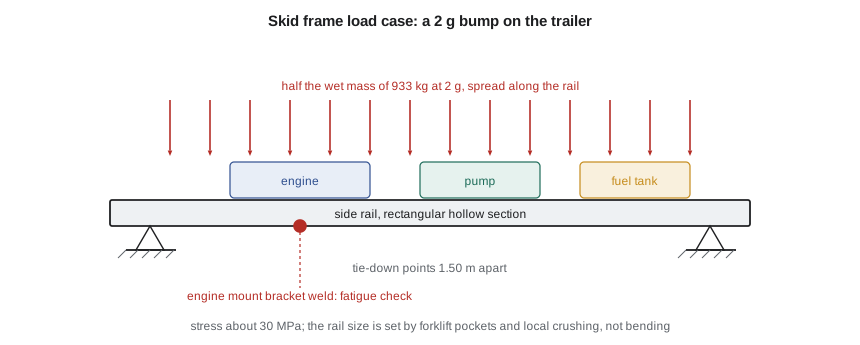
The frame is two rectangular hollow section rails joined by cross-members, carrying the engine, pump and tank. Its worst static load case is transport: the skid on its trailer hitting a pothole. The team took a vertical acceleration of 2 g, a common figure for road transport design of trailer-mounted equipment, and assumed the load shares equally between the rails, each spanning 1.50 m between tie-down points.
# TDX-150 frame: rail bending in transport, weld fatigue at the engine mount, and engine isolation
import math
g = 9.81
m_wet, span = 933.0, 1.50                        # kg, m between tie-down points
W = m_wet * g * 2.0 / 2                          # 2 g bump, shared by two rails (N)
M = W * span / 8 * 1000                          # uniform load, N mm
for B, H, t in ((76.0, 152.0, 6.4), (64.0, 127.0, 4.8)):   # rectangular hollow section rails, mm
    I = (B * H**3 - (B - 2*t) * (H - 2*t)**3) / 12           # mm^4
    Z = I / (H / 2)                                          # mm^3
    sigma = M / Z
    kgm = 7.85e-6 * (B * H - (B - 2*t) * (H - 2*t)) * 1000
    print(f"Rail {H:.0f} x {B:.0f} x {t}: Z = {Z / 1e3:5.1f} cm^3, {kgm:4.1f} kg/m, stress {sigma:4.1f} MPa, factor on 345 MPa {345 / sigma:4.1f}")
print(f"Bending moment per rail in a 2 g bump: {M / 1e6:.2f} kN m")

# Fatigue at the fillet-welded engine mount bracket: nominal stress range from +/- 0.5 g road vibration
SCF = 1.6                                        # bracket stiffness step at the weld toe (from the FE model)
d_sigma = 2 * 0.5 / 2.0 * sigma * SCF            # range for +/-0.5 g, scaled from the 2 g case
FAT, m = 71.0, 3                                 # IIW detail category: fillet weld toe, 2e6 cycles
N_allow = 2e6 * (FAT / d_sigma) ** m
cycles = 10 * 1000 * 3600 / 60 * 3.5             # 10 years x 1,000 km/yr at 60 km/h, 3.5 Hz body bounce
print(f"Stress range {d_sigma:.1f} MPa, allowable {N_allow:.2e} cycles, demand {cycles:.2e} -> damage {cycles / N_allow:.2f}")

# Engine on four rubber mounts: transmissibility at running and firing frequencies
fn, zeta = 9.0, 0.08
for name, f in (("shaft rotation 1,800 rpm", 30.0), ("3-cylinder firing", 45.0)):
    r = f / fn
    T = math.sqrt((1 + (2*zeta*r)**2) / ((1 - r*r)**2 + (2*zeta*r)**2))
print(f"{name:24s} {f:4.0f} Hz: r = {r:.2f}, transmissibility {T:.3f} ({(1 - T):.0%} isolation)")Rail 152 x 76 x 6.4: Z = 105.7 cm^3, 21.6 kg/m, stress 16.2 MPa, factor on 345 MPa 21.3 Rail 127 x 64 x 4.8: Z = 56.5 cm^3, 13.7 kg/m, stress 30.4 MPa, factor on 345 MPa 11.4 Bending moment per rail in a 2 g bump: 1.72 kN m Stress range 24.3 MPa, allowable 5.00e+07 cycles, demand 2.10e+06 -> damage 0.04 shaft rotation 1,800 rpm 30 Hz: r = 3.33, transmissibility 0.112 (89% isolation) 3-cylinder firing 45 Hz: r = 5.00, transmissibility 0.053 (95% isolation)
Even with the lighter 127 by 64 by 4.8 mm section, the bending stress is only about 30 MPa, a factor of 11 on yield. That looks wasteful, and Farah asked about it at the preliminary review. The answer is that bending does not govern this frame. The rails must be tall enough for forklift pockets, thick enough not to crush locally where a forklift tine or a tie-down strap bears on them, and stiff enough not to twist when the skid stands on uneven ground. Hannah's finite element model of the lifting eye and forklift pocket regions, using the techniques of the finite element course, showed peak stresses of about 140 MPa at the pocket corners under a forklift lift with a 2 g dynamic factor, well within the material's strength, and justified the thinner wall.
Fatigue in transport
Static strength is not the whole story. A skid that travels 1,000 km a year on rural roads sees millions of small load cycles, and the weak points are welds, where geometry and residual stress concentrate damage. The program checks the fillet weld at the engine mount bracket using the detail category approach of the International Institute of Welding recommendations, in which each weld geometry has a fatigue strength, its FAT class, at two million cycles, and an S-N slope of 3. The bracket's weld toe is treated as FAT 71 with a stress concentration factor of 1.6 from the finite element model.
With a stress range of about 24 MPa from road vibration of ±0.5 g, the weld could survive about 50 million cycles, against a demand of about 2.1 million over ten years, giving a Miner damage sum of 0.04. The margin is large, which is consistent with experience: well-made welded skids rarely fail in fatigue unless something resonates. That caveat pointed straight at the next analysis.
Vibration isolation
A three-cylinder four-stroke diesel at 1,800 rpm shakes at its rotation frequency of 30 Hz and, more strongly, at its firing frequency of 45 Hz, one and a half times the rotation frequency for a three-cylinder four-stroke. If those forces reach the frame and canopy, they cause noise, fatigue and loosening. The engine sits on four rubber mounts chosen to give a mounted natural frequency of about 9 Hz. The transmissibility of a single-degree-of-freedom isolator, from the vibrations course, gives about 11 percent of the force transmitted at 30 Hz and 5 percent at 45 Hz. The mounts also had to be checked for starting and stopping, when the engine passes slowly through 9 Hz; the rubber's damping limits the motion, and flexible connections on the exhaust, fuel and coolant lines accommodate it.
Lucie Arsenault, whose group did the vibration work on Tidewater's own packages, added one more check: that no frame or canopy panel had a natural frequency near 30 or 45 Hz. A quick modal run of Hannah's model found the lid panel of the canopy at 47 Hz. A single folded stiffening rib moved it to 68 Hz for 0.4 kg.
Worked problem
Changing engine speed at night
The TRIZ session suggested slowing the engine at night once the water level falls. By the affinity laws, what happens to flow, head and power at 1,500 rpm, and is the isolation still adequate?
Show solution
- Speed ratio 1,500/1,800 = 0.833.
- On a curve with mostly dynamic head, flow scales with speed and head with speed squared: flow about 75 L/s, head about 12.5 m; but with 9 m of static head, the real operating point falls further: solving the scaled pump curve against the system curve gives about 66 L/s at 13.8 m.
- Shaft power at the new point is about 13.5 kW, roughly 0.58 times the rated value, a large fuel saving.
- Rotation becomes 25 Hz and firing 37.5 Hz; frequency ratios to the 9 Hz mounts are 2.8 and 4.2, so transmissibility rises slightly to about 0.16 and 0.07, still acceptable.
Answer: Night speed cuts flow and fuel substantially and keeps isolation acceptable; the static head means flow falls more than the simple affinity law suggests.
Checking the checks
Every analysis was reviewed by someone who had not done it. Émilie rechecked Kwame's hydraulic numbers by hand. Owen checked the fatigue calculation against Tidewater's standard method and found that Kwame had used the stress amplitude rather than the stress range in his first version, which would have overstated life by a factor of eight. Errors like that are common and invisible to their author, which is why review is part of the analysis, not an afterthought.
Common mistakes
MistakeAnalyzing whatever the software can do rather than what the requirements need.
InsteadWrite an analysis plan linking each analysis to a requirement at risk.
MistakeReading the operating point from the pump curve alone.
InsteadFind it where the pump and system curves cross, for each lift and hose arrangement.
MistakeTreating NPSH available equal to NPSH required as acceptable.
InsteadKeep a margin; NPSHr marks a 3 percent head drop, not the absence of cavitation.
MistakeUsing stress amplitude in an S-N curve defined by stress range.
InsteadCheck which quantity the fatigue data use; a factor of two in stress is a factor of eight in life at slope 3.
MistakeAssuming a frame is oversized because bending stress is low.
InsteadCheck local crushing, forklift and lifting loads, stiffness and resonance before removing material.
Summary and key terms
- An analysis plan tied each analysis to a requirement at risk and to the simplest adequate method.
- The rated point, 90 L/s at 18 m, is where the 6.0 m lift system curve meets the pump curve.
- At 7.5 m lift NPSH available falls below NPSH required, so the pump primes but cavitates at full flow, justifying R-03.
- Engine load of about 24.3 kW uses about 6.8 L/h, giving 26.5 h from 180 L usable.
- Frame bending stress is about 30 MPa; local loads, stiffness and forklift pockets set the rail size.
- Weld fatigue damage over ten years is about 0.04, and 9 Hz engine mounts isolate 89 to 95 percent of engine forces.
- Operating point
- The flow at which pump head equals system head.
- System curve
- The head a piping system demands as a function of flow.
- Static head
- The part of system head from elevation differences, independent of flow.
- NPSH available
- The suction head above vapor pressure available at the pump inlet.
- NPSH required
- The suction head at which the pump's head drops by 3 percent from cavitation.
- Brake specific fuel consumption
- Fuel mass used per unit of engine work, in g/kWh.
- FAT class
- The fatigue strength of a weld detail at two million cycles.
- Miner's rule
- Fatigue damage summed as cycles applied divided by cycles to failure.
- Transmissibility
- The ratio of force transmitted through an isolator to the force applied.
- Affinity laws
- Scaling of pump flow, head and power with speed and impeller size.
Practice problems
Work each problem on paper first, then reveal the answer to check.
A pump gives H = 30 − 0.002 Q² and the system needs H = 10 + 0.0015 Q² (Q in L/s). Find the operating point.
Show answer
0.0035 Q² = 20, Q = 75.6 L/s, H = 18.6 m.
At sea level with 101.3 kPa, 6.5 m lift, 0.9 m suction losses and water at 20 °C (2.34 kPa), what is NPSHa?
Show answer
10.33 − 6.5 − 0.9 − 0.24 = 2.69 m.
An engine at 20 kW uses 240 g/kWh of diesel at 0.84 kg/L. Find the fuel use per hour.
Show answer
20 × 0.240 / 0.84 = 5.71 L/h.
A weld of FAT 80 sees a stress range of 40 MPa. Estimate its life with slope 3.
Show answer
2 × 10⁶ × (80/40)³ = 1.6 × 10⁷ cycles.
Mounts give 9 Hz; the disturbing frequency is 18 Hz. With light damping, is the engine isolated?
Show answer
r = 2, above √2, so force is reduced, but only to about 1/(4 − 1) = 0.33; isolation is modest.
Lesson quiz · 5 questions
Score 60% or more to complete this lesson.
Create a free account to save your progress, take quizzes and earn a certificate.