Energy and weighted-residual formulations

The bar and beam elements of the last two lessons could be derived from equilibrium of their nodes, because their exact behavior was known. That route closes as soon as the element is two- or three-dimensional, or the field varies in a way no simple formula describes. The finite element method's general foundation is a different one: instead of satisfying the governing differential equation at every point, which is impossible with a finite number of unknowns, it satisfies the equation in an average sense. This lesson develops the two classical ways of doing that, the energy (Rayleigh-Ritz) method and the weighted-residual (Galerkin) method, and shows how they lead to the same element matrices. It also shows how the error behaves as elements shrink, which is the basis of the convergence checks Owen will make on every real model.

Minimum potential energy

For a linear elastic body under fixed loads, the total potential energy is the strain energy stored in the body minus the work potential of the applied loads. For a bar it is

Among all displacement fields that satisfy the supports, called kinematically admissible fields, the true one makes Π a minimum. That is the principle of minimum potential energy. It turns a differential equation into a minimization problem, and minimization problems can be solved approximately by searching over a limited family of trial functions.

The Rayleigh-Ritz method

Lord Rayleigh and Walther Ritz, around the turn of the twentieth century, proposed choosing a trial function with a few unknown coefficients, \(u \approx a_1\phi_1(x) + a_2\phi_2(x) + \dots\), each \(\phi_i\) satisfying the supports, and choosing the coefficients to minimize Π. Setting \(\partial\Pi/\partial a_i = 0\) for each coefficient gives a set of linear equations \(Ka = f\), a stiffness matrix and load vector in miniature. The approximation is the best one within the chosen family in an energy sense, and since the true solution minimizes Π, the approximate structure is always too stiff: its strain energy and its displacements under a single load are underestimated. This bound is a valuable property, and it carries over to displacement-based finite elements.

Owen tries the method on the VT-12 column from Lesson 2. With the single trial function \(\phi_1 = x\), the displacement varies linearly down the column and the strain is constant. Minimizing Π gives \(a_1 = (wL^2/2 + PL)/(EAL)\). With two trial functions, x and x², the trial family contains the exact quadratic solution, and the Ritz method must find it.

# Rayleigh-Ritz and Galerkin solutions for a bar, and how the error falls as the mesh is refined
import math
E, A, L = 200e9, 3.60e-3, 6.0; w = A * 7850 * 9.81; P = 4500.0      # the VT-12 column from Lesson 2
EA = E * A
exact = lambda x: (P * x + w * (L * x - x * x / 2)) / EA
# Ritz 1: u = a1 x. Potential energy Pi = 1/2 EA a1^2 L - integral of w a1 x dx - P a1 L; dPi/da1 = 0
a1 = (w * L**2 / 2 + P * L) / (EA * L)
# Ritz 2: u = a1 x + a2 x^2 gives a 2x2 system K a = f
K = [[EA * L, EA * L**2], [EA * L**2, EA * 4 * L**3 / 3]]
f = [w * L**2 / 2 + P * L, w * L**3 / 3 + P * L**2]
det = K[0][0] * K[1][1] - K[0][1] * K[1][0]
b1 = (f[0] * K[1][1] - K[0][1] * f[1]) / det; b2 = (K[0][0] * f[1] - K[1][0] * f[0]) / det
for x in (3.0, 6.0):
    print(f"x = {x:.1f} m: exact {1e6*exact(x):.3f} um, one-term Ritz {1e6*a1*x:.3f} um, two-term Ritz {1e6*(b1*x + b2*x*x):.3f} um")
print(f"Top stress: exact {(P + w*L)/A/1e6:.4f} MPa, one-term {E*a1/1e6:.4f} MPa, two-term {E*b1/1e6:.4f} MPa")

# Galerkin with linear elements for -EA u'' = q(x) on 0 < x < 1, u(0) = u(1) = 0, with q = sin(pi x)
# Exact u = sin(pi x)/pi^2 (EA = 1). Compare nodal error, maximum error and the energy-norm error as h halves.
def galerkin(ne):
    h = 1.0 / ne; n = ne - 1
    diag, off = [2.0 / h] * n, [-1.0 / h] * (n - 1)
    # consistent load by 3-point Gauss quadrature on each element
    g = [(-math.sqrt(0.6), 5/9), (0.0, 8/9), (math.sqrt(0.6), 5/9)]
    F = [0.0] * (ne + 1)
    for e in range(ne):
        for xi, wt in g:
            x = (e + (xi + 1) / 2) * h; q = math.sin(math.pi * x)
            F[e] += wt * h / 2 * q * (1 - xi) / 2; F[e + 1] += wt * h / 2 * q * (1 + xi) / 2
    b = F[1:-1]
    # tridiagonal (Thomas) solve
    c, d = off[:], b[:]; dd = diag[:]
    for i in range(1, n):
        m = off[i-1] / dd[i-1]; dd[i] -= m * c[i-1]; d[i] -= m * d[i-1]
    u = [0.0] * n; u[-1] = d[-1] / dd[-1]
    for i in range(n - 2, -1, -1): u[i] = (d[i] - c[i] * u[i+1]) / dd[i]
    U = [0.0] + u + [0.0]
    nodal = max(abs(U[i] - math.sin(math.pi * i * h) / math.pi**2) for i in range(ne + 1))
    emax, en2 = 0.0, 0.0
    for e in range(ne):
        slope = (U[e+1] - U[e]) / h
        for k in range(21):
            x = (e + k / 20) * h; uh = U[e] + slope * (x - e * h)
            emax = max(emax, abs(uh - math.sin(math.pi * x) / math.pi**2))
        for xi, wt in g:
            x = (e + (xi + 1) / 2) * h; en2 += wt * h / 2 * (slope - math.cos(math.pi * x) / math.pi)**2
    return nodal, emax, math.sqrt(en2)
print("\nGalerkin, linear elements:  ne   nodal error   max error   energy error   energy ratio")
prev = None
for ne in (2, 4, 8, 16, 32):
    nod, em, en = galerkin(ne)
    r = f"{prev/en:6.2f}" if prev else "   -  "
    print(f"                            {ne:3d}   {nod:9.2e}   {em:9.2e}   {en:10.3e}      {r}")
    prev = en

x = 3.0 m: exact 23.948 um, one-term Ritz 22.215 um, two-term Ritz 23.948 um
x = 6.0 m: exact 44.431 um, one-term Ritz 44.431 um, two-term Ritz 44.431 um
Top stress: exact 1.7121 MPa, one-term 1.4810 MPa, two-term 1.7121 MPa

Galerkin, linear elements:  ne   nodal error   max error   energy error   energy ratio
                              2    4.26e-06    2.13e-02    9.796e-02         -  
                              4    6.08e-08    7.13e-03    5.051e-02        1.94
                              8    9.28e-10    1.91e-03    2.545e-02        1.98
                             16    1.44e-11    4.86e-04    1.275e-02        2.00
                             32    2.25e-13    1.22e-04    6.378e-03        2.00

The program shows both behaviors. The one-term solution gets the bottom displacement exactly, 44.431 µm, but halfway down it gives 22.215 µm instead of 23.948 µm, and its constant stress, 1.481 MPa, is the same 13.5 percent underestimate of the top stress that the one-element model gave in Lesson 2. That is no coincidence: one linear bar element is a one-term Ritz approximation with the shape function as the trial function. The two-term solution is exact everywhere. When the trial family contains the true solution, the Ritz method finds it.

From global trial functions to finite elements

The classical Ritz method uses trial functions that span the whole body, and finding suitable ones for a complicated shape is as hard as solving the original problem. The finite element method's insight is to use trial functions that are nonzero only over a few elements: the shape functions of each node, pieced together into a tent-shaped function that is one at its node and zero at every other node. Every such function automatically satisfies the supports if the restrained nodes are left out, and any shape can be meshed. Minimizing the potential energy over this family of piecewise functions gives exactly the assembled equations \(Ku = F\) of the direct stiffness method, now with a general recipe for the element matrices:

where N holds the shape functions, B their derivatives (the strain-displacement matrix), D the material stiffness, b the body force and t the surface traction. These two formulas generate every displacement-based element in this course and in commercial software, from the bar to the twenty-node brick. The consistent nodal loads of Lesson 2 are the second formula applied to a bar.

The Galerkin method

Not every problem has a potential energy to minimize, and the Galerkin method, named for Boris Galerkin, works directly with the differential equation. Write the equation as \(\mathcal{L}(u) = 0\); an approximate solution leaves a residual \(R = \mathcal{L}(u_h)\) that is not zero. The weighted-residual idea is to require that the residual vanish on average when multiplied by each of a set of weighting functions. Galerkin's choice is to use the trial functions themselves as the weights. For the bar equation \(-EAu'' = q\), multiplying by a weight w and integrating by parts gives

This is the weak form. It needs only first derivatives of u, so piecewise linear functions are acceptable, and its boundary term brings in the applied end forces naturally. With the shape functions as both trial and weighting functions, it gives the same element stiffness and consistent load as the energy method. For problems with a potential energy the two methods are equivalent; for others, such as heat conduction with convection or fluid flow, Galerkin's method still applies, which is why it is the more general foundation and the one most texts use.

How fast does the error fall?

The second part of the program solves a model problem with a known answer, \(-u'' = \sin \pi x\) on a unit bar with both ends fixed, whose exact solution is \(\sin(\pi x)/\pi^2\). It measures three kinds of error as the number of linear elements doubles from 2 to 32: the error at the nodes, the largest error anywhere, and the error in the energy norm, which measures the error in the derivative (strain) averaged over the bar.

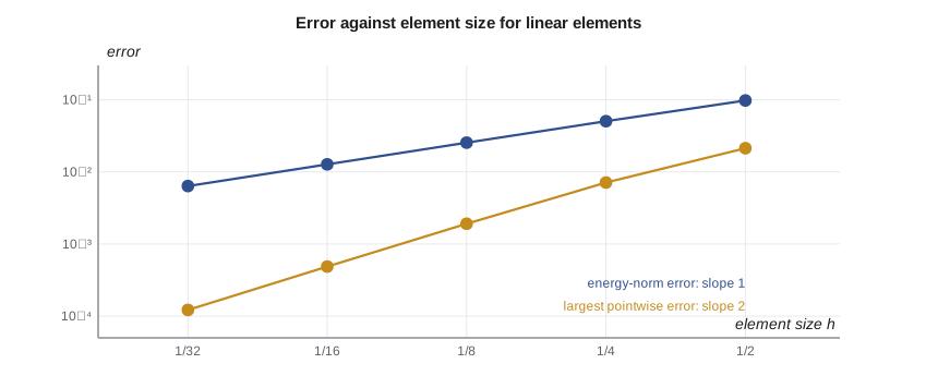
The nodal error is already tiny with two elements and falls to rounding level, the same nodal exactness seen in Lesson 2. The largest pointwise error falls by a factor of about four each time h halves, so it is proportional to h²; the energy-norm error falls by a factor of two, proportional to h. These rates are general for linear elements: displacement errors behave as h² and strain and stress errors as h. Quadratic elements improve both by one power, to h³ and h². On a log-log graph the error falls along a straight line whose slope is the order of convergence.

These rates are what make convergence studies meaningful. If an analyst refines a mesh and the stress changes by a factor consistent with the expected order, the results are in the asymptotic range and can be extrapolated; if it changes erratically or keeps growing, something else is going on, such as a singularity, a modeling error or elements too distorted to converge properly. Lesson 8 turns this into a practical procedure for the TP-80 shaft shoulder.

Requirements on elements

For the error to fall at all as elements shrink, the elements must satisfy two conditions. They must be complete: able to represent rigid-body motion and constant strain exactly, since as an element shrinks, the true field across it approaches a constant strain state. And they must be compatible: the displacement must be continuous between elements, without gaps or overlaps, to the order needed by the weak form (displacement for solids, displacement and slope for beams). Elements that violate these conditions can still be useful, and some well-known elements deliberately relax compatibility to improve bending behavior, but they must pass the patch test, a numerical check that a small patch of elements reproduces a constant strain state exactly. Software developers run such tests; users rarely need to, but should know that element quality is a tested property, not an assumption.