Dynamics: mass matrices and modal analysis

In the vibrations course Lucie Arsenault taught Owen to keep natural frequencies away from running speed and vane-pass frequency, and he found the TP-80's baseplate mode, its shaft's critical speed and the reed frequency of the VT-12 by hand formulas and tests. Those formulas cover simple shapes. The heavier-duty pump's baseplate, a fabricated frame on four isolators carrying a larger motor, has modes that no formula describes, and Lucie wants its first few natural frequencies predicted before it is built, so the design can be changed on paper rather than with stiffeners welded on in the field. This lesson extends the finite element method to vibration: the mass matrix, the eigenvalue problem it leads to, and the checks that confirm a modal model.

The equation of motion and the eigenvalue problem

Adding inertia to the static equation gives the finite element equation of motion, \(M\ddot{u} + C\dot{u} + Ku = F(t)\), where M is the mass matrix and C the damping matrix. For free, undamped vibration, the motion is harmonic, \(u = \phi\sin\omega t\), and substituting gives the generalized eigenvalue problem

Its solutions are pairs: a natural frequency \(\omega_i\) and a mode shape \(\phi_i\), one pair for each degree of freedom. In practice only the lowest few modes are wanted, those within or near the frequency range of the excitation, and solvers find them efficiently with subspace iteration or the Lanczos method, without computing all the rest. The modes are orthogonal with respect to both K and M, which is what allows the modal superposition method of the vibrations course: the response to any load is a combination of independent single-degree-of-freedom responses, one per mode.

Consistent and lumped mass

The mass matrix comes from the kinetic energy, using the same shape functions as the stiffness: \(M_e = \int \rho N^{\mathsf{T}}N\,dV\). This is the consistent mass matrix. For a bar element of mass m it is \((m/6)\begin{bmatrix} 2 & 1 \\ 1 & 2\end{bmatrix}\), and for a beam element of mass per length μ and length h it is the 4 by 4 matrix

The alternative, the lumped mass matrix, simply places half of each element's mass at each node, as point masses with no coupling between nodes and no rotary inertia. It is diagonal, which makes it cheap to store and invert and ideal for explicit dynamics such as crash and impact analysis. The consistent matrix is more accurate per element. The two err in opposite directions: displacement-based stiffness is too stiff (Lesson 5), and the consistent mass, derived consistently with it, keeps the frequencies too high; the lumped mass concentrates inertia at the nodes and usually brings frequencies down, often below the exact values.

Point masses for attached equipment are added directly to the diagonal of M at the nodes where they attach: an impeller at the end of a shaft, a motor on a baseplate, a valve on a pipe. For large components, rotary inertia should be included as well, and the attachment's stiffness matters as much as its mass.

Testing the method on the baseplate rail

Owen tests the method on a case with an exact answer: one side rail of the baseplate idealized as a simply supported beam 1.6 m long with EI = 1.72 MN·m², carrying a share of the equipment mass smeared along it so that its mass per length is 148 kg/m. The exact first natural frequency of a simply supported uniform beam, from the vibrations course, is \(f_1 = (\pi/L)^2\sqrt{EI/\mu}/2\pi = 66.15\) Hz. The program solves the eigenvalue problem by inverse iteration, which repeatedly solves \(Kx_{new} = Mx\) and normalizes, converging to the lowest mode, and then finds the frequency from the Rayleigh quotient \(\omega^2 = \phi^{\mathsf{T}}K\phi/\phi^{\mathsf{T}}M\phi\).

# Modal analysis by finite elements: consistent and lumped mass, inverse iteration, and the TP-80 shaft critical speed
import math
def solve(A, b):
    n = len(b); A = [r[:] for r in A]; b = b[:]
    for k in range(n):
        p = max(range(k, n), key=lambda i: abs(A[i][k])); A[k], A[p] = A[p], A[k]; b[k], b[p] = b[p], b[k]
        for i in range(k + 1, n):
            f = A[i][k] / A[k][k]
            if f:
                for j in range(k, n): A[i][j] -= f * A[k][j]
                b[i] -= f * b[k]
    x = [0.0] * n
    for i in range(n - 1, -1, -1): x[i] = (b[i] - sum(A[i][j] * x[j] for j in range(i + 1, n))) / A[i][i]
    return x
def lowest_mode(K, M, iters=200):
    """Inverse iteration: repeatedly solve K x_new = M x and normalize; returns omega^2 by the Rayleigh quotient."""
    n = len(K); x = [1.0] * n
    for _ in range(iters):
        y = [sum(M[i][j] * x[j] for j in range(n)) for i in range(n)]; x = solve(K, y)
        s = max(abs(v) for v in x); x = [v / s for v in x]
    Kx = [sum(K[i][j] * x[j] for j in range(n)) for i in range(n)]; Mx = [sum(M[i][j] * x[j] for j in range(n)) for i in range(n)]
    return sum(a * b for a, b in zip(x, Kx)) / sum(a * b for a, b in zip(x, Mx)), x
def beam(EI, mu, xs, lumped=False):
    n = len(xs); K = [[0.0] * (2*n) for _ in range(2*n)]; M = [[0.0] * (2*n) for _ in range(2*n)]
    for e in range(n - 1):
        h = xs[e+1] - xs[e]; c = EI / h**3; mm = mu * h / 420
        ke = [[12*c, 6*h*c, -12*c, 6*h*c], [6*h*c, 4*h*h*c, -6*h*c, 2*h*h*c], [-12*c, -6*h*c, 12*c, -6*h*c], [6*h*c, 2*h*h*c, -6*h*c, 4*h*h*c]]
        if lumped: me = [[mu*h/2, 0, 0, 0], [0, 0, 0, 0], [0, 0, mu*h/2, 0], [0, 0, 0, 0]]
        else: me = [[156*mm, 22*h*mm, 54*mm, -13*h*mm], [22*h*mm, 4*h*h*mm, 13*h*mm, -3*h*h*mm],
                    [54*mm, 13*h*mm, 156*mm, -22*h*mm], [-13*h*mm, -3*h*h*mm, -22*h*mm, 4*h*h*mm]]
        for a in range(4):
            for b in range(4): K[2*e + a][2*e + b] += ke[a][b]; M[2*e + a][2*e + b] += me[a][b]
    return K, M
def reduce(K, M, fixed):
    free = [i for i in range(len(K)) if i not in fixed]
    return [[K[a][b] for b in free] for a in free], [[M[a][b] for b in free] for a in free], free
# 1. Baseplate side rail as a simply supported beam: L = 1.6 m, EI = 1.72 MN m^2, smeared mass 148 kg/m
EI, mu, L = 1.72e6, 148.0, 1.6
f_exact = (math.pi / L)**2 * math.sqrt(EI / mu) / (2 * math.pi)
print(f"Rail, exact first natural frequency {f_exact:.2f} Hz")
print(" elements   consistent mass (Hz)   lumped mass (Hz)")
for ne in (1, 2, 4, 8):
    xs = [L * i / ne for i in range(ne + 1)]; res = []
    for lump in (False, True):
        K, M = beam(EI, mu, xs, lump)
        fixed = [0, 2*ne]
        if lump and ne == 1: res.append(float('nan')); continue    # one lumped element has no free mass
        Kr, Mr, free = reduce(K, M, fixed)
        if lump:   # rotational DOF carry no mass: condense them out statically before the eigen solve
            tr = [i for i, d in enumerate(free) if d % 2 == 0]; ro = [i for i, d in enumerate(free) if d % 2 == 1]
            Krr = [[Kr[a][b] for b in ro] for a in ro]
            Kc = [[Kr[a][b] - sum(Kr[a][r] * solve(Krr, [Kr[rr][b] for rr in ro])[k] for k, r in enumerate(ro)) for b in tr] for a in tr]
            Kr, Mr = Kc, [[Mr[a][b] for b in tr] for a in tr]
        w2, _ = lowest_mode(Kr, Mr); res.append(math.sqrt(w2) / (2 * math.pi))
    print(f"   {ne:2d}        {res[0]:10.2f}            " + (f"{res[1]:10.2f}" if res[1] == res[1] else "     -"))
# 2. TP-80 shaft (uniform 35 mm idealization of Lesson 4) with the 9.5 kg impeller at the overhang end
E, d = 200e9, 0.035; EIs = E * math.pi * d**4 / 64; mus = 7850 * math.pi * d**2 / 4
xs = [0.0, 0.05, 0.10, 0.15, 0.20, 0.24, 0.28, 0.32, 0.36]
K, M = beam(EIs, mus, xs); M[2*(len(xs)-1)][2*(len(xs)-1)] += 9.5
Kr, Mr, free = reduce(K, M, [0, 8])
w2, mode = lowest_mode(Kr, Mr); f1 = math.sqrt(w2) / (2 * math.pi)
k_tip = 3 * EIs / (0.16**2 * 0.36)
f_sdof = math.sqrt(k_tip / 9.5) / (2 * math.pi)
print(f"\nShaft: one-mass estimate {f_sdof:.1f} Hz = {60*f_sdof:.0f} rpm; FE with shaft mass {f1:.1f} Hz = {60*f1:.0f} rpm")
print(f"Running speed 1,760 rpm is {100*1760/(60*f1):.0f} percent of the first critical speed")
# 3. Two-degree-of-freedom check by the Jacobi rotation method (package on pads, on a frame), M^-1/2 K M^-1/2
m1, m2, k1, k2 = 120.0, 310.0, 12e6, 8.8e6        # frame and package masses (kg), frame and pad stiffness (N/m)
a, b, c = (k1 + k2) / m1, -k2 / math.sqrt(m1 * m2), k2 / m2
th = 0.5 * math.atan2(2 * b, a - c)
l1 = a * math.cos(th)**2 + 2 * b * math.sin(th) * math.cos(th) + c * math.sin(th)**2
l2 = a * math.sin(th)**2 - 2 * b * math.sin(th) * math.cos(th) + c * math.cos(th)**2
fs = sorted(math.sqrt(v) / (2 * math.pi) for v in (l1, l2))
print(f"Two-mass model by one Jacobi rotation: {fs[0]:.1f} Hz and {fs[1]:.1f} Hz")

Rail, exact first natural frequency 66.15 Hz
 elements   consistent mass (Hz)   lumped mass (Hz)
    1             73.42                 -
    2             66.41                 65.67
    4             66.16                 66.13
    8             66.15                 66.15

Shaft: one-mass estimate 113.1 Hz = 6785 rpm; FE with shaft mass 111.0 Hz = 6660 rpm
Running speed 1,760 rpm is 26 percent of the first critical speed
Two-mass model by one Jacobi rotation: 19.6 Hz and 68.7 Hz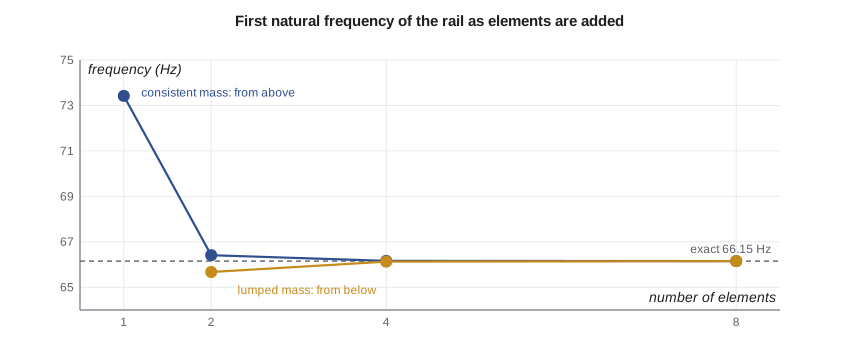

With one consistent element the first frequency is 73.4 Hz, 11 percent high; with two it is within 0.4 percent, and with four it is essentially exact. The lumped results come from below, 65.7 Hz with two elements, and also converge by four. A lumped model with a single element has no free mass at all, since the element's masses sit at the two supports, which is a useful reminder that lumped models need enough nodes for the mass to move. For lumped beam models the rotation degrees of freedom have no mass, so the program first condenses them out of the stiffness matrix, a step called static condensation that software performs automatically.

The bracketing behavior is useful in practice. If a consistent and a lumped model of the same mesh give frequencies close together, both are probably converged; if they differ widely, the mesh is too coarse for that mode. Higher modes, with more half-waves along the member, need proportionally more elements: as a rule of thumb, at least four to six elements per half-wave of the highest mode of interest.

The TP-80 shaft critical speed

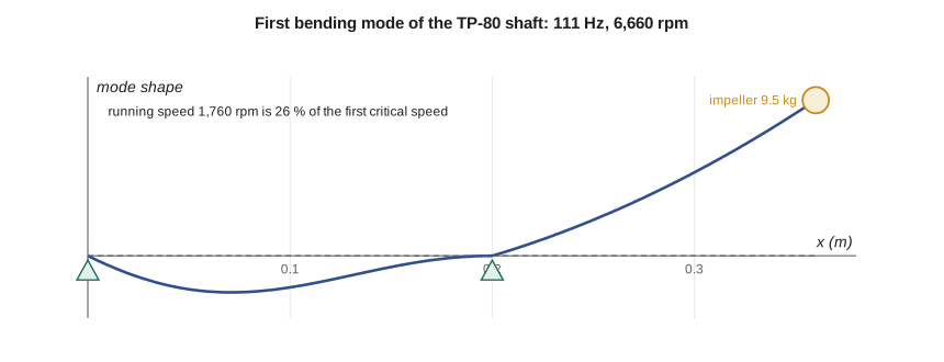
In Lesson 4 the uniform-shaft model gave a stiffness of 4.80 MN/m at the impeller. Treating the 9.5 kg impeller as a single mass on that spring gives a first natural frequency of 113.1 Hz, or 6,785 rpm, the estimate from machine design of about 6,800 rpm. The finite element model, with eight beam elements carrying the shaft's own mass and the impeller as a point mass, gives 111.0 Hz, 6,660 rpm, about two percent lower because the shaft's mass now takes part in the motion. Running speed, 1,760 rpm, is 26 percent of the first critical speed, so the TP-80 is a stiff-shaft machine with a wide margin. For the heavier-duty version, with a longer overhang and a heavier impeller, the margin will shrink, and Owen will repeat the calculation with the stepped geometry, bearing stiffness and, following the vibrations course, an allowance for the water's added mass and the seal's stiffness.

Two masses and the Jacobi method

The last part of the program returns to Lesson 1's spring model, now with masses: the frame top, 120 kg, on its 12 MN/m stiffness, and the 310 kg package on the 8.8 MN/m pads. The 2 by 2 eigenvalue problem is solved by one Jacobi rotation, the classical method that zeros an off-diagonal term of a symmetric matrix by rotating its coordinates; for a 2 by 2 matrix one rotation suffices, while larger matrices need repeated sweeps. The frequencies are 19.6 Hz, mostly the package bouncing on its pads with the frame helping, and 68.7 Hz, the frame and package moving against each other. The single-mass estimate from the vibrations course, 26.8 Hz for the package on its pads alone, was too high because it treated the frame as rigid. Including the frame's flexibility moves the first mode from 26.8 Hz to 19.6 Hz, further below the 29.3 Hz running speed. That eases the near-resonance found in the vibrations course but changes the isolation calculation, and it is a reminder that every component in the load path affects a natural frequency.

Damping and response

The eigenvalue problem gives frequencies and shapes but not amplitudes. Amplitudes need the damping and the excitation. Damping is rarely modeled element by element; instead, a modal damping ratio is assigned to each mode, typically from test or experience, such as 2 to 5 percent for welded steel structures, as the vibrations course discussed. Harmonic response analysis then gives the amplitude at each frequency of a sinusoidal load such as unbalance, and transient analysis gives the response to a time history such as a start-up or a shock. Both are built on the modes, so a sound modal model, with its frequencies checked, is the foundation of every dynamic analysis.