Bar elements and assembly

The spring of Lesson 1 had a stiffness given in advance. Real parts are made of material with a modulus, a cross-section and a length, and the first element derived from those properties is the bar: a straight member that carries only axial load. Bars appear everywhere in pump work. A vertical turbine pump hangs its bowl assembly from a column pipe; a tie rod holds a motor stool; a bolt is a bar in tension. Owen's example in this lesson is the VT-12, Tidewater's vertical turbine pump, whose 6 m column he met in the vibrations course when its reed frequency had to be kept away from running speed. This time the question is static: how far does the column stretch, and what is the stress at the top flange, when it hangs under its own weight and carries the bowl assembly?

Deriving the bar element

Consider a bar element of length L, cross-sectional area A and Young's modulus E, with nodes 1 and 2 at its ends and axial displacements \(u_1\) and \(u_2\). Assume that the displacement varies linearly along the element. With a local coordinate x running from 0 at node 1 to L at node 2, the displacement is

The functions \(N_1\) and \(N_2\) are the shape functions of the element. Each equals one at its own node and zero at the other, so the nodal values are the actual displacements at the nodes. Every element in this course is built the same way: choose shape functions, use them to express the field inside the element in terms of nodal values, and derive the element matrices from them.

The strain is the derivative of the displacement, \(\varepsilon = du/dx = (u_2 - u_1)/L\), constant along the element, and the stress is \(\sigma = E\varepsilon\). The axial force \(EA(u_2 - u_1)/L\) acts on node 2 in the negative direction and on node 1 in the positive direction, which gives the element stiffness matrix

This is the spring matrix with \(k = EA/L\), the familiar axial stiffness of a bar. The bar element adds two things to the spring: a way to recover stress from the displacements, and a way to represent loads distributed along the element, such as self weight.

Distributed loads and consistent nodal forces

Finite element equations only have forces at nodes, so a load distributed along an element must be converted into equivalent nodal forces. The rule that does this consistently comes from the principle of virtual work, which Lesson 5 develops: the nodal force at node i is the integral of the distributed load multiplied by that node's shape function. For a uniform load q per unit length on a linear bar element this gives \(qL/2\) at each node, the obvious answer of splitting the load equally. For a linearly varying load the split is unequal, and for higher-order elements the consistent loads are sometimes counterintuitive. Software calculates these automatically from pressures, gravity or body forces, but an analyst checking a model should know that the total of the nodal loads must equal the total applied load.

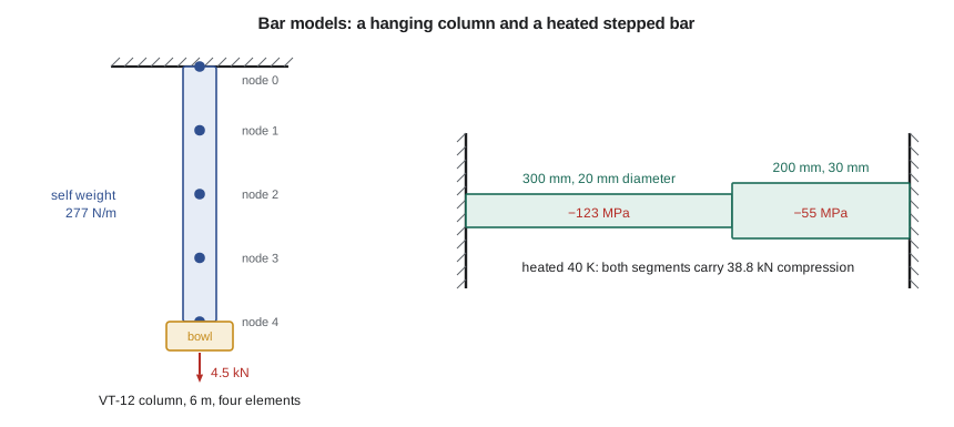
For the VT-12 column the distributed load is the pipe's own weight. The column is DN150 steel pipe with a cross-sectional area of 3.60 × 10⁻³ m², so it weighs \(A\rho g = 3.60 \times 10^{-3} \times 7850 \times 9.81 = 277\) N/m, about 1.66 kN over 6 m. The bowl assembly, impellers and bowls hanging at the bottom, weighs 4.5 kN. Water inside the column and the hydraulic down-thrust of the impellers are carried by other paths in this pump, so Owen leaves them out for this check. The top flange is node 0 and is fixed.

Exact at the nodes, approximate between them

The exact solution is easy to find by hand. At a distance x below the flange the column carries the bowl plus the weight of the pipe below that point, \(N(x) = P + w(L - x)\). Integrating the strain \(N/EA\) gives the displacement, and at the bottom

which is 0.0444 mm, or 44 µm. The stress at the top, where the force is greatest, is \((P + wL)/A = 1.712\) MPa. Both are tiny, as expected for a heavy-walled pipe; the purpose here is to learn how the element behaves, not to find a problem with the column.

# Bar elements: the VT-12 column pipe hanging under its own weight, and a heated bar between rigid supports
def solve(A, b):
    n = len(b); A = [r[:] for r in A]; b = b[:]
    for k in range(n):
        p = max(range(k, n), key=lambda i: abs(A[i][k])); A[k], A[p] = A[p], A[k]; b[k], b[p] = b[p], b[k]
        for i in range(k + 1, n):
            f = A[i][k] / A[k][k]
            for j in range(k, n): A[i][j] -= f * A[k][j]
            b[i] -= f * b[k]
    x = [0.0] * n
    for i in range(n - 1, -1, -1): x[i] = (b[i] - sum(A[i][j] * x[j] for j in range(i + 1, n))) / A[i][i]
    return x

E, A, L = 200e9, 3.60e-3, 6.0               # steel column pipe: Pa, m^2, m
w = A * 7850 * 9.81                          # self weight per meter, N/m
P = 4500.0                                   # bowl assembly hanging at the bottom, N
def column(ne):
    n = ne + 1; h = L / ne; K = [[0.0] * n for _ in range(n)]; F = [0.0] * n
    for e in range(ne):
        k = E * A / h
        for a, b, v in ((e, e, k), (e + 1, e + 1, k), (e, e + 1, -k), (e + 1, e, -k)): K[a][b] += v
        F[e] += w * h / 2; F[e + 1] += w * h / 2          # consistent load: half the element weight to each node
    F[-1] += P
    u = [0.0] + solve([r[1:] for r in K[1:]], F[1:])   # node 0 (top flange) is fixed
    stress_top = E * (u[1] - u[0]) / h                 # element 1 stress (constant in the element)
    return u[-1], stress_top
exact_tip = P * L / (E * A) + w * L**2 / (2 * E * A)
exact_top = (P + w * L) / A
print(f"Self weight {w:.1f} N/m; exact bottom displacement {1e3*exact_tip:.4f} mm; exact stress at top {exact_top/1e6:.3f} MPa")
print(" elements   bottom u (mm)   error     stress in top element (MPa)   error")
for ne in (1, 2, 4, 8, 16):
    tip, s = column(ne)
    print(f"   {ne:3d}      {1e3*tip:10.4f}   {100*(tip-exact_tip)/exact_tip:6.3f} %         {s/1e6:8.3f}                 {100*(s-exact_top)/exact_top:6.2f} %")

# Heated stepped bar held between rigid walls: steel, 300 mm of 20 mm diameter then 200 mm of 30 mm, heated 40 K
import math
alpha, dT = 12e-6, 40.0
segs = [(0.300, math.pi * 0.020**2 / 4), (0.200, math.pi * 0.030**2 / 4)]
K = [[0.0] * 3 for _ in range(3)]; F = [0.0] * 3
for e, (Le, Ae) in enumerate(segs):
    k = E * Ae / Le; ft = E * Ae * alpha * dT              # thermal load vector [-ft, +ft]
    for a, b, v in ((e, e, k), (e + 1, e + 1, k), (e, e + 1, -k), (e + 1, e, -k)): K[a][b] += v
    F[e] -= ft; F[e + 1] += ft
u1 = F[1] / K[1][1]                                       # nodes 0 and 2 fixed, only node 1 free
for e, (Le, Ae) in enumerate(segs):
    ua, ub = (0.0, u1) if e == 0 else (u1, 0.0)
    sig = E * ((ub - ua) / Le - alpha * dT)
    print(f"Segment {e+1}: stress {sig/1e6:7.1f} MPa, force {sig*Ae/1e3:6.2f} kN")
print(f"Step displacement {1e3*u1:.4f} mm (negative: toward the wall of the thinner segment)")

Self weight 277.2 N/m; exact bottom displacement 0.0444 mm; exact stress at top 1.712 MPa
 elements   bottom u (mm)   error     stress in top element (MPa)   error
     1          0.0444    0.000 %            1.481                 -13.49 %
     2          0.0444    0.000 %            1.597                  -6.75 %
     4          0.0444    0.000 %            1.654                  -3.37 %
     8          0.0444    0.000 %            1.683                  -1.69 %
    16          0.0444    0.000 %            1.698                  -0.84 %
Segment 1: stress  -123.4 MPa, force -38.78 kN
Segment 2: stress   -54.9 MPa, force -38.78 kN
Step displacement -0.0411 mm (negative: toward the wall of the thinner segment)

The first table holds a surprise. Every mesh, even a single element, gives the bottom displacement exactly. This is a known property of the linear bar element with consistent loads: for one-dimensional problems of this kind, the finite element nodal values coincide with the exact solution at the nodes, whatever the number of elements. Between the nodes, though, the element can only vary linearly, while the true displacement is quadratic, and the stress, which the element takes as constant, is wrong. A single element reports 1.481 MPa for the stress in the top element, 13.5 percent low, because it gives the average stress over the whole column. Each halving of the element size halves the error, to 0.84 percent with sixteen elements.

Two lessons follow that apply far beyond bars. The first is that displacements are more accurate than stresses. Stress depends on the derivative of the displacement, and differentiating an approximation loses accuracy; finite element displacements typically converge one order faster than stresses. The second is that a constant-stress element reports something like the average stress over its length, so where the stress varies steeply, as it does at a fillet or a hole, coarse elements underestimate the peak. Lesson 8 returns to this when it considers the shaft shoulder.

Assembly with several elements

With n elements there are n + 1 nodes. Element e joins nodes e and e + 1, so its four stiffness terms go into rows and columns e and e + 1 of the global matrix. The result is tridiagonal, with nonzero terms only on and next to the diagonal. Most of a large finite element matrix is likewise zero, because each node is connected only to its neighbors, and solvers exploit that sparsity to handle very large models. The numbering of nodes affects how the nonzero terms are arranged, and older solvers needed the nodes renumbered to keep them close to the diagonal. Modern packages do this automatically.

Thermal loads and statically indeterminate bars

A bar whose temperature rises by ΔT wants to expand by \(\alpha \Delta T L\). If it is free, it simply does so and carries no stress. If it is held, it develops stress. The finite element treatment adds an initial strain \(\varepsilon_0 = \alpha \Delta T\): the stress becomes \(\sigma = E(\varepsilon - \varepsilon_0)\), and the effect appears as a pair of equivalent nodal forces \(\mp EA\alpha\Delta T\) that push the element's ends apart. Commercial codes handle thermal loads this way, usually taking the temperature field from a thermal analysis of the same mesh, which Lesson 10 covers.

The second model in the program is a stepped steel rod, 300 mm of 20 mm diameter followed by 200 mm of 30 mm diameter, held between rigid walls and heated by 40 K. It is statically indeterminate: equilibrium alone says only that both segments carry the same force, and compatibility, the condition that the total length cannot change, is needed to find it. The finite element method handles indeterminate structures with no extra effort, since compatibility is built into the shared nodal displacements. The program finds a compressive force of 38.8 kN in both segments, with stresses of −123 MPa in the thin segment and −55 MPa in the thick one. The step between them moves 0.041 mm toward the thinner segment's wall, because the stiffer thick segment pushes harder. A hand check: if the rod were uniform and fully restrained, the stress would be \(E\alpha\Delta T = 200\,000 \times 12 \times 10^{-6} \times 40 = 96\) MPa. The thin segment's stress is higher and the thick segment's lower, with the force in between, as expected.

Heated parts held between stiff supports are common in pump work: a hot-water pump's casing anchored at both nozzles, a stainless shaft sleeve on a steel shaft, a bolt that heats up less than the flange it clamps. In each case the thermal stress depends on the stiffness of everything in the load path, which is why the finite element model must include, or represent by springs, the parts that provide the restraint.

Applying the idea to a pump part

Owen's real use of bar elements on the heavier-duty TP-80 is modest but typical: the four tie rods that clamp the bearing frame to the casing adapter. A full three-dimensional model of the frame could include the rods as solid cylinders, but representing each one as a bar element joining the two parts, preloaded by an initial strain, gives nearly the same stiffness for a tiny fraction of the cost. Choosing the simplest element that captures the behavior that matters is a skill developed through practice, and it starts with understanding what each element can and cannot represent.