Wind energy

Wind has become one of the largest sources of new electricity in North America, and the prairies and upper Midwest have some of the best wind resources on the continent. Minnesota was an early wind state; wind now supplies roughly a quarter of its generation, and more is planned to meet the 2040 standard. Kofi has been approached by a developer who proposes that Northgate sign a long-term power purchase agreement for the output of a share of a new wind farm, to match the electricity its future heat pumps will use. Before the team can judge the offer, it needs to understand how much energy a wind turbine really produces and what limits it.

The power in the wind

Air of density \(\rho\) moving at speed \(v\) through an area \(A\) carries kinetic energy at the rate

The cube of the speed is the most important fact in wind energy. Doubling the wind speed multiplies the available power by eight. A site with an average speed 10 percent higher has roughly a third more power in the wind. Density matters too: cold, dense prairie air in January carries about 15 percent more power than warm summer air at the same speed.

A turbine cannot extract all of this power, because the air must keep moving to leave the rotor. Momentum theory for an ideal rotor shows that the maximum fraction that can be extracted, the Betz limit, is 16/27, or 59.3 percent, reached when the rotor slows the wind to one third of its upstream speed in the far wake. The ratio of the power extracted to the power in the wind is the power coefficient \(C_p\). Modern three-bladed turbines reach a \(C_p\) of about 0.45 to 0.50 at their best operating point, and the whole drivetrain, including gearbox, generator and converter, loses a few percent more.

The power curve

A turbine's power curve shows its electrical output against wind speed at hub height. Below the cut-in speed, about 3 m/s, it does not run. Between cut-in and the rated speed, about 10 to 12 m/s, output rises roughly with the cube of speed as the control system adjusts rotor speed to keep \(C_p\) near its maximum. Above rated speed the blades are pitched to shed power and hold output at the generator's rating. At the cut-out speed, typically 25 m/s, the turbine shuts down to protect itself, although many modern machines ramp output down gradually rather than stopping abruptly.

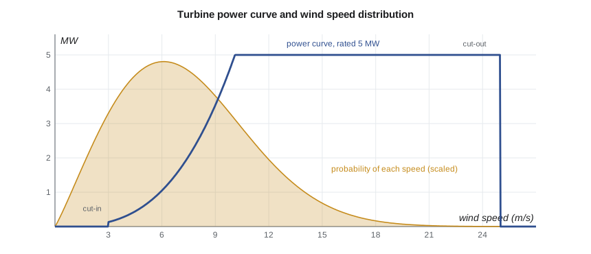
Turbines have grown steadily. Land-based machines installed in North America now commonly have rotors of 130 to 170 m diameter on towers over 100 m tall, rated at 3 to 6 MW. Larger rotors on the same generator lower the rated speed and raise the capacity factor, because the turbine reaches full output more often. Taller towers reach faster, steadier wind, because wind speed increases with height above the ground, roughly with a power law of exponent about 0.14 to 0.25 depending on terrain and stability.

Wind speed distribution and annual energy

Wind speed varies continuously. Over a year the distribution of hourly mean speeds at a site is usually well described by a Weibull distribution with a shape factor \(k\) of about 2 and a scale factor \(c\) a little above the mean speed.

The annual energy is the power curve weighted by the distribution and multiplied by 8,760 hours. In practice developers measure wind with met masts and remote-sensing lidar for at least a year, correlate the measurements with long-term reference data, and calculate energy with the manufacturer's power curve for the site's air density. They then subtract losses: wake losses from turbines shading each other, typically 5 to 12 percent on a large farm, availability losses for maintenance and faults, electrical losses, blade icing and curtailment when the grid cannot take the power.

# Wind energy: Betz limit, a turbine power curve and annual energy from a Weibull wind speed distribution
SITE = 'us'
import math
rho = 1.22                         # air density, kg/m3 (cold prairie air is denser than this in winter)
D = 150.0; A = math.pi*D**2/4      # rotor diameter, m
P_rated = 5.0e6                    # W
def curve(v):
    if v < 3.0 or v > 25.0: return 0.0
    p = 0.5*rho*A*0.45*v**3        # power coefficient 0.45 below rated
    return min(p, P_rated)
v_r = (P_rated/(0.5*rho*A*0.45))**(1/3)
print(f"Rotor {D:.0f} m, swept area {A:,.0f} m2; rated {P_rated/1e6:.0f} MW reached at about {v_r:.1f} m/s")
print(f"Betz limit 16/27 = {16/27:.3f}; this turbine's Cp below rated: 0.45")
# Weibull distribution at hub height: shape k, scale c
k, c = {'ca': (2.1, 8.3), 'us': (2.2, 8.6)}[SITE]
vmean = c*math.gamma(1 + 1/k)
dv = 0.1; E = 0.0
for i in range(int(30/dv)):
    v = (i + 0.5)*dv
    f = (k/c)*(v/c)**(k - 1)*math.exp(-(v/c)**k)
    E += curve(v)*f*dv
E_yr = E*8760/1e9          # GWh gross
loss = 0.12                # wakes, availability, icing, curtailment, electrical
print(f"Weibull k {k}, c {c} m/s -> mean speed {vmean:.2f} m/s")
print(f"Gross annual energy {E_yr:.1f} GWh; net after {loss*100:.0f} % losses {E_yr*(1-loss):.1f} GWh")
print(f"Net capacity factor {E_yr*(1-loss)*1000/(P_rated/1e6*8760):.2f}")
# Cube law: what a 10 % change in mean speed does
for f in (0.9, 1.1):
    c2 = c*f; E2 = 0.0
    for i in range(int(30/dv)):
        v = (i + 0.5)*dv; ff = (k/c2)*(v/c2)**(k - 1)*math.exp(-(v/c2)**k); E2 += curve(v)*ff*dv
    print(f"  mean speed x {f:.1f}: energy x {E2/E:.2f}")
# Turbines needed for Northgate's planned heat pump electricity (80 GWh/yr)
print(f"Turbines to supply 80 GWh/yr on an annual basis: {80/(E_yr*(1-loss)):.1f}")

Rotor 150 m, swept area 17,671 m2; rated 5 MW reached at about 10.1 m/s
Betz limit 16/27 = 0.593; this turbine's Cp below rated: 0.45
Weibull k 2.2, c 8.6 m/s -> mean speed 7.62 m/s
Gross annual energy 20.7 GWh; net after 12 % losses 18.2 GWh
Net capacity factor 0.42
  mean speed x 0.9: energy x 0.84
  mean speed x 1.1: energy x 1.14
Turbines to supply 80 GWh/yr on an annual basis: 4.4

Two results deserve attention. The capacity factor of about 0.4 is typical of good modern sites on the plains. And a 10 percent increase in mean wind speed raises energy by only about 14 percent, not 33 percent, because the turbine spends more of its time at rated output, where extra wind speed adds nothing. The cube law describes the wind; the power curve describes the machine.

Variability and the grid

Wind output varies from minute to minute with gusts, from hour to hour with weather systems, and from season to season. Over a large region, the output of many farms is smoother than that of one, but calm periods lasting several days still occur, often during the high-pressure systems that bring the coldest winter weather. For Northgate this matters directly: a wind farm that produces, on average, the electricity its heat pumps use will produce much less than that during some of the coldest, stillest weeks of the year, when heat demand is highest.

An annual power purchase agreement for wind is therefore an accounting match, not a physical one. In the hours when the wind farm produces more than Northgate uses, the surplus goes into the grid; when it produces less, Northgate draws on the grid. Whether that deal actually reduces emissions depends on whether the wind farm is additional, built because of the contract, and on what grid plants the wind displaces in each hour. A stronger approach, now adopted by some large buyers, is to match consumption with clean supply hour by hour, which requires storage, flexible demand or a mix of sources.

The grid also has limits on how much variable output it can absorb. Transmission must carry wind power from windy rural areas to cities; system operators need reserves and flexible plant to balance it; and in some hours wind farms are curtailed because there is nowhere for the power to go. Minnesota's grid is part of a large regional market whose operator balances wind across many states, and transmission expansion is one of the main constraints on further growth.

Capacity credit

System planners need to know how much a wind farm contributes to meeting the peak, not just how much energy it produces. The measure is its capacity credit, often estimated as its effective load-carrying capability: the amount of firm, always-available capacity that would give the system the same reliability as the wind farm. Because the coldest winter peaks often coincide with calm weather, the capacity credit of wind on a winter-peaking northern grid can be well below its capacity factor, sometimes 10 to 20 percent of its rating, and it falls as more wind is added because the farms' outputs are correlated. A planning study that counts wind's nameplate capacity toward the peak will badly overstate the system's reliability; one that counts its capacity credit will see why firm capacity, storage and flexible demand remain necessary even on grids with a great deal of wind.

Other considerations

Wind farms need land, but the turbines occupy only a small part of it; farming continues between them. They affect birds and bats, especially at poorly sited farms on migration routes, and careful siting, curtailment at low wind speeds when bats are active, and new detection systems reduce the effect. Noise and the moving shadows of blades limit how close turbines can be to homes, and local acceptance is often the deciding factor in whether a farm is built. In cold climates, ice on the blades reduces output and can be thrown from rotating blades, so turbines have ice detection and sometimes blade heating, and setbacks from roads and buildings. At the end of a turbine's 20 to 30 year life most of it can be recycled, although composite blades remain a challenge.

Offshore wind, with larger turbines and steadier winds, is growing on the Atlantic coast and in Europe but is not relevant to the prairies. Small turbines on buildings in cities produce very little energy because the wind there is slow and turbulent, and they should not be part of a serious plan.

The team concludes that a wind contract is a reasonable way for Northgate to support new clean generation and to fix part of its electricity cost for twenty years, and on the Minnesota grid it brings forward the carbon benefit of electrification before the grid as a whole reaches the 2040 standard. The contract does not provide firm capacity, so the heat pumps still need the grid and storage in calm weather.