
MEC-440 · Lesson 4 of 12 · 21 min
Cogeneration and district energy
Cogeneration, also called combined heat and power, is the technology Northgate was built on. A cogeneration plant makes electricity and uses the heat that a condensing plant would throw away. In MEC-330 the team analyzed a gas turbine with a heat recovery boiler and found a primary energy saving of about 23 percent over separate production. It also found that the carbon case for cogeneration depends on the grid: on the Minnesota grid of the day, cogeneration displaced fossil-fired power and cut emissions, so the team recommended building it. The board has asked the team to revisit that decision with a 2040 horizon, and to size any cogeneration properly against the network's load.
Why cogeneration saves fuel
Separate production makes electricity in a power plant at perhaps 40 to 55 percent efficiency and heat in a boiler at about 90 percent. A cogeneration plant uses one fuel input to make both: a gas engine might turn 42 percent of its fuel into electricity and recover 44 percent as useful heat from its jacket water and exhaust, a total of 86 percent. The heat it recovers is the heat that a condensing power plant would have rejected to a river. The saving is real, but it is not as large as the 86 percent total suggests, because electricity and heat are not equally valuable. A kilowatt-hour of electricity can drive a heat pump that delivers three kilowatt-hours of heat; a kilowatt-hour of 90 °C water cannot make electricity at all.
Three measures are in common use. Fuel utilization, or total efficiency, is the sum of electrical and useful thermal output divided by fuel input; it is easy to compute and flatters cogeneration because it adds heat and electricity as if they were equal. Primary energy saving compares the fuel used by cogeneration with the fuel that separate production of the same electricity and heat would need, using reference efficiencies for each. Exergy efficiency, introduced in MEC-330, weights the heat by its Carnot factor, which gives the most physically meaningful measure but is less used in regulation.
The primary energy saving formula, used in European regulation and widely in engineering studies, depends heavily on the reference efficiencies. Choose a reference power plant that is 35 percent efficient and cogeneration looks wonderful; choose a 60 percent combined cycle and the saving shrinks. A careful study states its references and justifies them.
Sizing on the load duration curve
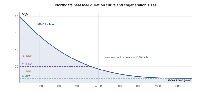
A load duration curve sorts the hours of the year by heat demand, from highest to lowest. The area under the curve is the annual heat. Any plant that runs whenever there is demand, up to its capacity, delivers the area under the curve and below its capacity line. Small plants run almost all year; larger plants add capacity that is used for fewer and fewer hours.
# Cogeneration for Northgate: sizing on the heat load duration curve, primary energy saving and CO2 against the grid
SITE = 'us'
import math
peak, annual = 80.0, 210.0            # MW and GWh of heat delivered
# hourly heat demand as a smooth load duration curve: q(h) = base + (peak - base) * (1 - h/8760)^k
base = 6.0
k = (peak - base)*8760/(annual*1000 - base*8760) - 1
def q(h): return base + (peak - base)*(1 - h/8760)**k
print(f"Load duration curve: base {base:.0f} MW, peak {peak:.0f} MW, shape exponent {k:.2f}")
eta_e, eta_h = 0.42, 0.44            # gas engine CHP: electrical and recovered heat efficiencies (HHV)
for size_th in (6, 12, 20, 30):
    heat = sum(min(q(h + 0.5), size_th) for h in range(8760))/1000      # GWh of CHP heat
    hours = heat*1000/size_th
    fuel = heat/eta_h; elec = fuel*eta_e
    print(f"  CHP heat {size_th:2d} MW (electric {size_th*eta_e/eta_h:4.1f} MW): heat {heat:5.1f} GWh, {hours:5.0f} full-load hours, power {elec:5.1f} GWh")
# Primary energy saving of the 12 MW-heat unit (reference: 0.90 boiler, 0.50 power plant)
eta_ref_h, eta_ref_e = 0.90, 0.50
pes = 1 - 1/(eta_h/eta_ref_h + eta_e/eta_ref_e)
print(f"\nPrimary energy saving: 1 - 1/({eta_h}/{eta_ref_h} + {eta_e}/{eta_ref_e}) = {pes:.3f}")
# CO2 per MWh of CHP electricity, crediting the boiler heat it displaces
gas_ef = 0.181
co2_per_MWh_e = (1/eta_e)*gas_ef*1000 - (eta_h/eta_e)*(gas_ef*1000/0.90)
print(f"Net CO2 per MWh of CHP power after heat credit: {co2_per_MWh_e:.0f} kg")
grid_now = {'ca': 0.002, 'us': 0.304}[SITE]
print(f"Grid factor today ({'Manitoba' if SITE=='ca' else 'Minnesota'}): {grid_now*1000:.0f} kg/MWh")
heat12 = sum(min(q(h + 0.5), 12) for h in range(8760))/1000
elec12 = heat12/eta_h*eta_e
for yr, g in ({'ca': ((2026, 0.002), (2035, 0.002), (2040, 0.002)), 'us': ((2026, 0.304), (2030, 0.22), (2035, 0.12), (2040, 0.0))}[SITE]):
    saving = elec12*1000*(g*1000 - co2_per_MWh_e)/1000          # t/yr (positive = CHP saves CO2)
    print(f"  {yr}: grid {g*1000:4.0f} kg/MWh -> CHP changes CO2 by {-saving:+8,.0f} t/yr")
print(f"Break-even grid factor: {co2_per_MWh_e:.0f} kg/MWh")Load duration curve: base 6 MW, peak 80 MW, shape exponent 3.12 CHP heat 6 MW (electric 5.7 MW): heat 52.6 GWh, 8760 full-load hours, power 50.2 GWh CHP heat 12 MW (electric 11.5 MW): heat 87.3 GWh, 7279 full-load hours, power 83.4 GWh CHP heat 20 MW (electric 19.1 MW): heat 120.8 GWh, 6038 full-load hours, power 115.3 GWh CHP heat 30 MW (electric 28.6 MW): heat 151.9 GWh, 5063 full-load hours, power 145.0 GWh Primary energy saving: 1 - 1/(0.44/0.9 + 0.42/0.5) = 0.247 Net CO2 per MWh of CHP power after heat credit: 220 kg Grid factor today (Minnesota): 304 kg/MWh 2026: grid 304 kg/MWh -> CHP changes CO2 by -6,981 t/yr 2030: grid 220 kg/MWh -> CHP changes CO2 by +22 t/yr 2035: grid 120 kg/MWh -> CHP changes CO2 by +8,359 t/yr 2040: grid 0 kg/MWh -> CHP changes CO2 by +18,364 t/yr Break-even grid factor: 220 kg/MWh
The results show the classic trade-off. A 6 MW unit, sized to the summer base load, runs every hour of the year but supplies only a quarter of the annual heat. A 12 MW unit runs about 7,300 full-load hours and supplies over 40 percent. Beyond about 20 MW the extra capacity runs too few hours to justify its capital. Many district heating systems size cogeneration to supply 40 to 60 percent of annual heat, with boilers for the peak, and add a hot-water storage tank so the units can run at full output when electricity prices are high and store the heat for later. Lesson 11 returns to storage.
The carbon question
When a cogeneration plant runs, it burns more gas than a boiler would to make the same heat, and it makes electricity that displaces generation somewhere on the grid. Whether it saves carbon depends on what it displaces. Crediting the heat at the boiler's emissions, the engine's net carbon per megawatt-hour of electricity is about 220 kg in this study. If the displaced grid electricity emits more than that, cogeneration saves carbon; if less, cogeneration adds carbon.
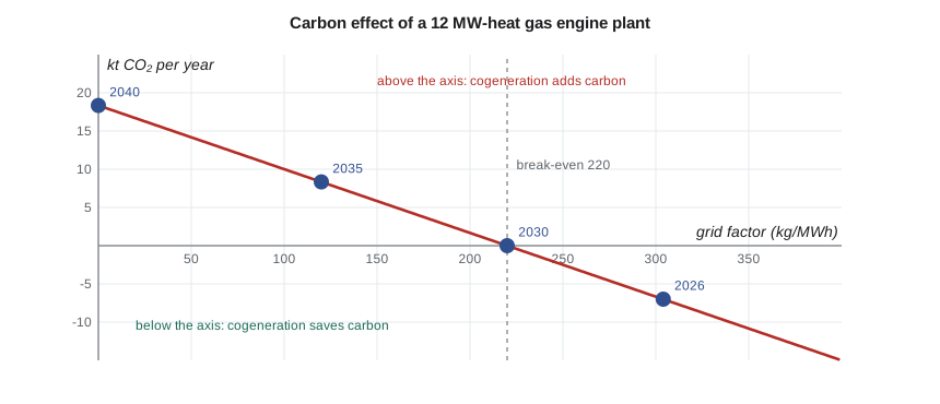
On today's Minnesota grid at about 300 kg/MWh, a 12 MW-heat engine plant would save about 7,000 t of carbon dioxide a year. But the grid is changing. If it follows the path the 2040 standard implies, the break-even point arrives around 2030, and after that the same plant adds emissions, about 18,000 t a year by 2040. An engine plant built in 2027 with a 25-year life would therefore save carbon for only its first few years. The team revises the MEC-330 recommendation: cogeneration on natural gas is a bridge, not a destination, and it should be built only if it can be paid for in a few years or converted to a low-carbon fuel.
The lesson here is general. Any decision about a long-lived plant should be tested against the grid of its whole life, not the grid of the year it is built. Marginal emissions add a further complication: the gas plants that cogeneration displaces on the margin may run for years after the average grid has become much cleaner. A study that uses the average factor will undervalue cogeneration in the short term; a study that uses today's marginal factor for 25 years will overvalue it. The honest approach is to show both and explain the choice.
District energy systems
Cogeneration and district energy have grown up together. District heating networks distribute hot water, or in older systems steam, through insulated pipes to many buildings. They let a city use heat sources that no single building could: cogeneration, waste-to-energy plants, industrial waste heat, large heat pumps drawing on rivers or sewage, deep geothermal wells, biomass boilers and seasonal storage. District cooling networks distribute chilled water from central chillers, sometimes using lake or river water directly.
Network technology has evolved in generations. The first generation used steam, as Northgate's older downtown loop still does. The second and third used pressurized hot water above 100 °C. Fourth-generation networks, the target of most new projects, supply water at about 50 to 70 °C, which lets them use heat pumps and low-grade waste heat efficiently and cuts distribution losses. The cost of that change is in the buildings, which must be able to heat with lower water temperatures, and MEC-430's health center was designed for exactly that, with 55/40 °C heating water.
| Generation | Typical supply temperature | Main heat sources | Distribution losses |
|---|---|---|---|
| First | Steam, 150 to 250 °C | Coal and gas boilers, cogeneration | High, 20 to 30 % |
| Second and third | 90 to 130 °C hot water | Cogeneration, waste-to-energy, biomass | 10 to 20 % |
| Fourth | 50 to 70 °C | Heat pumps, waste heat, solar thermal, storage | 5 to 10 % |
| Fifth (ambient loops) | 10 to 25 °C | Building-level heat pumps sharing a loop | Very low |
Return temperature is the network operator's most important design variable after supply temperature. Every degree of cooling achieved in the buildings increases the network's capacity for the same pipe sizes and flow, lowers pumping energy, reduces heat losses in the return pipes, and raises the efficiency of the plant that heats the water. Cogeneration engines with flue gas condensers, heat pumps and solar collectors all perform better with cooler return water. Northgate therefore requires its customers' substations to meet a maximum return temperature and charges a penalty when they do not, a practice common in Scandinavian networks.
Policy and markets
In the United States, the Public Utility Regulatory Policies Act of 1978 created qualifying facilities, including efficient cogeneration plants, and required utilities to interconnect with them and buy their power at the utility's avoided cost. The rules have been revised since, and in areas with competitive wholesale markets cogeneration sells into the market instead. Minnesota's utilities and regulators set the terms for interconnection and standby service, which can decide whether a project pays. In both countries, standby charges, the fees a utility levies for being ready to supply a customer when its own plant is down, are a frequent obstacle, and every cogeneration study should check them early.
Worked problem
Primary energy saving with different references
A gas engine cogeneration plant is 42 percent electrically efficient and recovers 44 percent of its fuel as useful heat (higher heating value). Calculate its fuel utilization and its primary energy saving with a reference boiler at 90 percent and a reference power plant at (a) 50 percent and (b) 35 percent.
Show solution
- Fuel utilization: \(0.42 + 0.44 = 0.86\).
- (a) \(\text{PES} = 1 - 1/(0.44/0.90 + 0.42/0.50) = 1 - 1/(0.489 + 0.840) = 1 - 0.752 = 0.248\).
- (b) \(\text{PES} = 1 - 1/(0.489 + 1.200) = 1 - 0.592 = 0.408\).
Answer: Fuel utilization is 86 percent. The primary energy saving is about 25 percent against an efficient gas-fired reference and about 41 percent against an old coal plant. The reference matters as much as the plant.
Tomás adds the result to the pathway model. Pathway A in lesson 12 will include gas cogeneration only where it makes sense on the local grid, and every pathway will be tested with and without it.
Common mistakes
MistakeQuoting fuel utilization as if it were efficiency.
InsteadUse primary energy saving or exergy, and state the reference efficiencies.
MistakeSizing cogeneration to the peak heat demand.
InsteadSize it on the load duration curve for many running hours, with boilers and storage for the peak.
MistakeJudging a 25-year plant against today's grid alone.
InsteadTest the carbon case against the projected grid over the plant's life.
MistakeForgetting standby and interconnection charges.
InsteadCheck the local utility's rules early in the study.
MistakeDesigning a low-temperature network for buildings that need hot water at 80 °C.
InsteadPlan building conversions with the network so return temperatures stay low.
Summary and key terms
- Cogeneration recovers heat a power plant would reject, saving fuel compared with separate production.
- Fuel utilization flatters cogeneration; primary energy saving depends on the reference efficiencies chosen.
- Units sized on the load duration curve to supply 40 to 60 percent of annual heat run many hours and pay back best.
- Cogeneration saves carbon only when the grid it displaces emits more than its own net carbon per kilowatt-hour, about 220 kg/MWh in this study.
- On the Minnesota grid gas cogeneration saves carbon now but adds it after about 2030 as the grid cleans up.
- Fourth-generation district heating at 50 to 70 °C suits heat pumps and waste heat but needs low-temperature buildings.
- Cogeneration
- Simultaneous production of electricity and useful heat from one fuel input; also called combined heat and power.
- Fuel utilization
- Electrical plus useful thermal output divided by fuel input.
- Primary energy saving
- Fraction of fuel saved by cogeneration compared with separate production using stated reference efficiencies.
- Load duration curve
- A plot of demand in each hour of the year sorted from highest to lowest.
- Full-load hours
- Annual energy from a plant divided by its rated capacity.
- Break-even grid factor
- The grid emission factor at which cogeneration neither adds nor saves carbon.
- Standby charge
- A fee for the utility being ready to supply a customer when its own generation is out of service.
- Fourth-generation district heating
- Networks supplying water at about 50 to 70 °C, suited to heat pumps and waste heat.
Practice problems
Work each problem on paper first, then reveal the answer to check.
A turbine cogeneration plant is 32 percent electric and 48 percent thermal. Find its fuel utilization and its primary energy saving with references of 90 percent and 50 percent.
Show answer
Utilization 0.80; \(\text{PES} = 1 - 1/(0.533 + 0.640) = 0.148\).
A 10 MW-heat unit supplies 70 GWh a year. How many full-load hours does it run?
Show answer
7,000 hours.
If the engine's net carbon is 220 kg/MWh and the grid factor is 150 kg/MWh, does cogeneration save or add carbon, and by how much per MWh of electricity?
Show answer
It adds about 70 kg per MWh of electricity.
Why do fourth-generation networks have lower distribution losses?
Show answer
The lower supply temperature reduces the temperature difference to the ground.
Why should a cogeneration study show both average and marginal grid factors?
Show answer
The plants displaced at the margin may emit far more than the average, especially in the early years.
Lesson quiz · 5 questions
Score 60% or more to complete this lesson.
Create a free account to save your progress, take quizzes and earn a certificate.