Multi-degree-of-freedom systems and modal analysis

A customer's TM-4 boiler feed pump, driven at 3,560 rpm by a two-pole motor through a gear-type coupling, has worn out two couplings in a year. The coupling teeth show polishing and pitting, but alignment checks are good and lateral vibration on the bearings is low. Lucie suspects torsional vibration, which a bearing housing sensor does not see (Lesson 2). The drive train has three significant inertias: the motor rotor, the coupling hubs and sleeve, and the pump rotor with its four impellers. Owen must find its torsional natural frequencies and mode shapes and check them against the torques that could excite them. Three degrees of freedom are too many for the hand methods of Lesson 8, so this lesson develops the general matrix approach, which works for any number.

The general eigenvalue problem

For n degrees of freedom the undamped free vibration equations are \(\mathbf{M}\ddot{\mathbf{x}} + \mathbf{K}\mathbf{x} = \mathbf{0}\), and harmonic solutions lead, as in Lesson 8, to the generalized eigenvalue problem

There are n natural frequencies ω_i and n mode shapes φ_i. For a torsional chain of inertias J₁, J₂, J₃ joined by shafts of stiffness k₁ and k₂, the matrices are

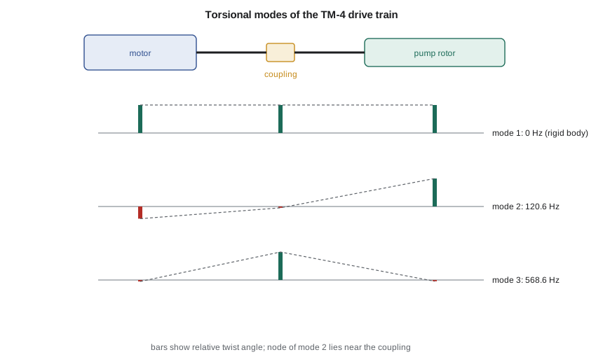
Because the chain is not attached to ground, K is singular, and one natural frequency is zero: the whole train can turn as a rigid body, which is of course what it does when it runs. The rigid-body mode is the reason the first frequency printed by the program is 0.0 Hz with all three mode shape values equal.

Solving the eigenvalue problem numerically

For two degrees of freedom, a determinant and a quadratic suffice. For more, a numerical method is used. A clean approach for symmetric problems is to transform to standard form. With \(\mathbf{x} = \mathbf{M}^{-1/2}\mathbf{q}\), the problem becomes \(\mathbf{A}\mathbf{q} = \omega^2\mathbf{q}\) with \(\mathbf{A} = \mathbf{M}^{-1/2}\mathbf{K}\mathbf{M}^{-1/2}\), a symmetric matrix. For a diagonal mass matrix, M^(−1/2) is just the diagonal of 1/√J_i. The Jacobi method then applies a sequence of plane rotations, each chosen to zero one off-diagonal element, until A is diagonal. The diagonal elements are the eigenvalues ω_i², and the accumulated rotations are the eigenvectors. The method is simple, robust and accurate for small matrices; finite element programs use more efficient methods, such as Lanczos iteration, for thousands of degrees of freedom, but the idea is the same.

# Torsional modes of the TM-4 drive train: motor rotor, coupling hub and pump rotor
import math
J = [0.48, 0.035, 0.21]             # polar inertias, kg m^2: motor, coupling, pump rotor
kt = [3.1e5, 1.15e5]                # shaft stiffnesses, N m/rad: motor shaft, coupling + pump shaft
def torsional_modes(J, kt):
    """Natural frequencies (Hz) and mode shapes of a three-inertia chain by the Jacobi method."""
    n = 3
    K = [
        [kt[0], -kt[0], 0.0],
        [-kt[0], kt[0] + kt[1], -kt[1]],
        [0.0, -kt[1], kt[1]],
    ]
    # Mass-normalize: A = M^-1/2 K M^-1/2 is symmetric, so the Jacobi method applies
    s = [1 / math.sqrt(j) for j in J]
    A = [ [K[i][k] * s[i] * s[k] for k in range(n)] for i in range(n)]
    V = [ [1.0 if i == k else 0.0 for k in range(n)] for i in range(n)]
    for sweep in range(50):
        off = sum(A[i][k]**2 for i in range(n) for k in range(n) if i != k)
        if off < 1e-18: break
        for p in range(n):
            for q in range(p + 1, n):
                if abs(A[p][q]) < 1e-30: continue
                th = 0.5 * math.atan2(2 * A[p][q], A[q][q] - A[p][p])
                c, sn = math.cos(th), math.sin(th)
                for k in range(n):        # rotate columns p, q
                    akp, akq = A[k][p], A[k][q]
                    A[k][p], A[k][q] = c * akp - sn * akq, sn * akp + c * akq
                for k in range(n):        # rotate rows p, q
                    apk, aqk = A[p][k], A[q][k]
                    A[p][k], A[q][k] = c * apk - sn * aqk, sn * apk + c * aqk
                for k in range(n):
                    vkp, vkq = V[k][p], V[k][q]
                    V[k][p], V[k][q] = c * vkp - sn * vkq, sn * vkp + c * vkq
    order = sorted(range(n), key=lambda i: A[i][i])
    modes = []
    for idx in order:
        lam = max(A[idx][idx], 0.0)
        phi = [V[i][idx] * s[i] for i in range(n)]        # back to physical coordinates
        big = max(phi, key=abs); phi = [p / big for p in phi]
        modes.append((math.sqrt(lam) / 2 / math.pi, phi))

    return modes

modes = torsional_modes(J, kt); n = 3
for f, phi in modes:
    print(f"Mode at {f:7.1f} Hz: motor {phi[0]:+.3f}, coupling {phi[1]:+.3f}, pump {phi[2]:+.3f}")
# Orthogonality: phi_i^T M phi_j = 0 for i != j
p1, p2 = modes[1][1], modes[2][1]
print(f"Check phi1' M phi2 = {sum(J[i]*p1[i]*p2[i] for i in range(n)):.2e} (zero within rounding)")
# Excitation check: running speed and vane pass (7 vanes per stage) against mode 2
f_run = 3560 / 60
for name, fe in (("1x running", f_run), ("2x line, 60 Hz grid", 120.0), ("vane pass 7x", 7 * f_run)):
    near = min(modes[1:], key=lambda m: abs(m[0] - fe))[0]
    print(f"{name:20s} {fe:6.1f} Hz: nearest torsional mode {near:6.1f} Hz, separation {abs(near-fe)/fe:5.1%}")
# Fix: a softer elastomeric coupling lowers mode 2 well below 120 Hz
for kc in (1.15e5, 0.60e5, 0.35e5):
    f2 = torsional_modes(J, [kt[0], kc])[1][0]
    print(f"coupling + shaft stiffness {kc/1e3:5.0f} kN m/rad: mode 2 at {f2:6.1f} Hz, separation from 120 Hz {abs(f2-120)/120:5.1%}")

Mode at     0.0 Hz: motor +1.000, coupling +1.000, pump +1.000
Mode at   120.6 Hz: motor -0.434, coupling -0.048, pump +1.000
Mode at   568.6 Hz: motor -0.053, coupling +1.000, pump -0.045
Check phi1' M phi2 = -3.69e-18 (zero within rounding)
1x running             59.3 Hz: nearest torsional mode  120.6 Hz, separation 103.2%
2x line, 60 Hz grid   120.0 Hz: nearest torsional mode  120.6 Hz, separation  0.5%
vane pass 7x          415.3 Hz: nearest torsional mode  568.6 Hz, separation 36.9%
coupling + shaft stiffness   115 kN m/rad: mode 2 at  120.6 Hz, separation from 120 Hz  0.5%
coupling + shaft stiffness    60 kN m/rad: mode 2 at   93.1 Hz, separation from 120 Hz 22.4%
coupling + shaft stiffness    35 kN m/rad: mode 2 at   73.5 Hz, separation from 120 Hz 38.8%

The program finds the rigid-body mode, a second mode at 120.6 Hz and a third at 568.6 Hz. In the second mode the motor and pump rotors twist against each other: normalized to the pump, the motor moves −0.43 and the coupling −0.05, so the node lies close to the coupling, where the twisting is concentrated. In the third mode the light coupling hubs oscillate between the two heavy rotors, which hardly move. The excitation check shows the problem at once. Running speed, 59.3 Hz, and the vane-pass frequency of the seven-vane impellers, 415 Hz, are well separated from both modes, but twice line frequency, 120 Hz, is within half a percent of the second mode.

Where does a 120 Hz torque come from?

An induction motor's electromagnetic torque is not perfectly steady. Any imbalance in the supply voltages, or asymmetry in the motor, produces a torque pulsation at twice line frequency: 120 Hz on the 60 Hz grids of Canada and the United States. Its amplitude is usually small, but a lightly damped torsional mode at 120.6 Hz amplifies it many times. Gear couplings add little damping. The polished and pitted teeth are the signature of an alternating torque large enough to slide the teeth against each other hundreds of times a second. Lucie confirms the diagnosis with a strain-gauge telemetry system on the coupling spacer, which shows an alternating torque at 120 Hz of about 30 percent of the running torque.

Orthogonality and modal coordinates

The mode shapes of a symmetric system have a powerful property: they are orthogonal with respect to both the mass and stiffness matrices,

The program checks the first of these numerically: the product for modes 2 and 3 is of the order of 10⁻¹⁸, zero within rounding. Orthogonality means that the modes can be used as a set of independent coordinates. Writing \(\mathbf{x} = \sum_i \boldsymbol{\phi}_i q_i(t)\) and premultiplying by φ_jᵀ uncouples the equations:

Each mode behaves as an independent single-degree-of-freedom system with its own modal mass, modal stiffness and modal force. All the results of Lessons 2 to 7 apply to each mode separately, and the physical response is the sum of the modal responses. This is modal superposition, the basis of most structural dynamics software. With damping, the equations uncouple exactly if the damping matrix is proportional to M and K (Rayleigh damping), and approximately if damping is light, which is why engineers usually assign a damping ratio to each mode.

The modal force φ_jᵀF tells which forces can excite which modes. A torque applied at the motor excites mode 2 in proportion to the motor's mode shape value, −0.43; the same torque applied at a node would not excite the mode at all. Likewise, a sensor placed at a node would not see it. Mode shapes therefore guide both the search for the cause and the choice of measurement point.

Experimental modal analysis

The modes of real structures are measured by experimental modal analysis. An instrumented hammer or a shaker excites the structure, accelerometers record the response at many points, and an analyzer computes the frequency response function between each input and output. Each resonance peak gives a natural frequency; its width gives the damping (the half-power method of Lesson 4); and the relative heights and signs of the peaks at different points give the mode shape. Tidewater uses impact modal tests on every new baseplate design and on the TM-4 casing, and compares the results with finite element models. Agreement within a few percent validates the model for use in later design changes. For torsional systems, which are hard to excite and measure directly, the calculated model, checked against a measured torque or speed fluctuation, is usually what engineers rely on.

The fix: retune the drive train

Moving the second mode away from 120 Hz can be done by changing an inertia or a stiffness. Adding inertia to the coupling would do little, since mode 2 is dominated by the two rotors. Changing the coupling stiffness is effective, because the twisting in mode 2 is concentrated across it. The last lines of the program show the effect of replacing the gear coupling with an elastomeric coupling. Reducing the combined coupling and pump shaft stiffness from 115 to 60 kN·m/rad moves mode 2 to 93.1 Hz, 22 percent below 120 Hz and 57 percent above running speed. A still softer coupling, 35 kN·m/rad, moves it to 73.5 Hz, but that is only 24 percent above running speed and close to the range in which start-up transients could excite it. Owen recommends the 60 kN·m/rad coupling, whose rubber elements also add damping.

Lateral modes and the limits of lumped models

The same matrix approach handles lateral vibration of a rotor, a pipe system or a baseplate, with the coordinates now being displacements and rotations at chosen nodes. As the number of nodes increases, the lumped model approaches the continuous system of Lesson 10. Lucie's practical guidance is to use at least four to six nodes per half-wavelength of the highest mode of interest, and to check that adding nodes no longer changes the frequencies of interest. The TM-4's lateral rotordynamic model in Lesson 11 uses forty-eight shaft elements for exactly this reason.