
MEC-380 · Lesson 12 of 12 · 25 min
Vibration measurement, condition monitoring and the capstone
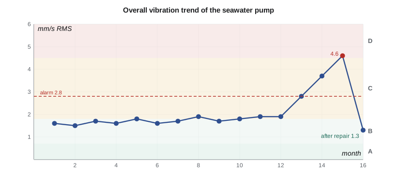
The last lesson brings Owen back to Casco Point Seafoods. Besides the brine pump on the platform of Lesson 8, the plant runs a second TP-80 as its seawater supply pump in the wharf pump house, on a skid bolted to the concrete deck. The plant's maintenance contractor measures it monthly with a portable data collector, and the overall vibration has climbed over three months from 1.9 to 4.6 mm/s RMS. The plant manager wants to know whether the pump is about to fail, what is wrong with it, and what to do. Lucie hands the case to Owen as his capstone: he must take measurements, analyze them, diagnose the faults using everything in the course, recommend repairs, and verify the result. First, though, he needs to understand the instruments and the signal processing behind the numbers.
Transducers
Three kinds of sensor dominate machinery vibration work. Piezoelectric accelerometers, the most common, contain a crystal loaded by a small mass; the crystal's charge is proportional to acceleration. They are small, rugged and work from a few hertz to well above 10 kHz, and most include built-in electronics to condition the signal. Their useful upper frequency is limited by their own mounted resonance, which depends strongly on how they are attached: a stud mount gives the highest, a magnet a lower one and a hand-held probe tip the lowest, often only 1 to 2 kHz. Velocity transducers, either moving-coil types or accelerometers with built-in integration, measure velocity directly. Proximity probes are non-contacting eddy-current sensors mounted in the bearing housing and aimed at the shaft; they measure the shaft's motion relative to the bearing and are standard on machines with oil-film bearings, such as large multistage pumps and turbines, where the shaft can move a lot within a housing that hardly moves.
Measurements are taken in three directions at each bearing: horizontal, vertical and axial. The comparison between directions is itself diagnostic. Unbalance gives similar horizontal and vertical amplitudes, about 90° apart in phase; misalignment gives high axial vibration and 2×; looseness gives very different amplitudes in different directions. A consistent measurement point, marked on the machine, is essential for trending, because readings can change by 50 percent between nearby points.
From signal to spectrum
A data collector samples the transducer signal at a rate f_s and records N samples, a time window of length N/f_s. The spectrum is computed by the fast Fourier transform (FFT), which decomposes the record into components at frequencies spaced by the resolution \(\Delta f = f_s/N\), up to the Nyquist frequency f_s/2. Signals above f_s/2 would fold back as false lower frequencies (aliasing), so collectors filter them out before sampling. Two choices control what the spectrum can show. The maximum frequency must cover the forcing frequencies of interest: bearing defect frequencies and their harmonics, vane pass, gear mesh. The resolution must separate components that are close together: running speed from twice line frequency in a motor, or a bearing harmonic from vane pass in a pump. Finer resolution needs a longer record.
Because a component rarely falls exactly on a frequency line, the record is multiplied by a window function, commonly the Hann window, which tapers the ends to zero. The window reduces leakage of energy into distant lines, at the cost of spreading each component over a few lines and reducing its peak height by up to about 15 percent if it falls between lines. Collectors usually average several spectra to reduce random noise. The overall vibration, the number used for alarm levels and severity zones, is the RMS value of the signal over a specified band, typically 10 to 1,000 Hz for velocity.
# Condition monitoring of the Casco Point Seafoods brine pump: spectrum, bearing frequencies and severity
import math, cmath, random
fr = 1760 / 60                              # shaft speed, Hz
# Rolling bearing defect frequencies for the 6307 drive-end bearing (approximate geometry)
nb, d, D, phi = 8, 13.49, 57.5, 0.0         # balls, ball and pitch diameters (mm), contact angle
ratio = d / D * math.cos(phi)
freqs = {'1x': fr, '2x': 2 * fr, '6x vane pass': 6 * fr,
         'BPFO': nb / 2 * fr * (1 - ratio), 'BPFI': nb / 2 * fr * (1 + ratio),
         'BSF': D / (2 * d) * fr * (1 - ratio**2), 'FTF': fr / 2 * (1 - ratio)}
for k in ('BPFO', 'BPFI', 'BSF', 'FTF'):
    print(f"{k}: {freqs[k]:6.2f} Hz = {freqs[k]/fr:.3f} x running speed")
# Synthetic velocity signal (mm/s) standing in for the field recording
fs, N = 2048, 16384                         # 8 s record, resolution 0.125 Hz
random.seed(7)
comps = [(fr, 4.40, 0.3), (2 * fr, 0.70, 1.1), (freqs['BPFO'], 0.55, 0.2), (2 * freqs['BPFO'], 0.35, 2.0),
         (6 * fr, 0.90, 0.7)]
x = []
for i in range(N):
    t = i / fs
    x.append(sum(a * math.sqrt(2) * math.sin(2 * math.pi * f * t + p) for f, a, p in comps) + random.gauss(0, 0.25))
overall = math.sqrt(sum(v * v for v in x) / N)
print(f"\nOverall velocity {overall:.2f} mm/s RMS ({overall*math.sqrt(2)/25.4:.3f} in/s peak)")
def fft(a):                                 # recursive radix-2 FFT
    n = len(a)
    if n == 1: return a
    ev, od = fft(a[0::2]), fft(a[1::2])
    out = [0] * n
    for k in range(n // 2):
        tw = cmath.exp(-2j * math.pi * k / n) * od[k]
        out[k], out[k + n // 2] = ev[k] + tw, ev[k] - tw
    return out
w = [0.5 - 0.5 * math.cos(2 * math.pi * i / N) for i in range(N)]   # Hann window
X = fft([complex(x[i] * w[i]) for i in range(N)])
amp = [2 * abs(X[k]) / (N * 0.5) / math.sqrt(2) for k in range(N // 2)]   # RMS amplitude per bin
sw2 = sum(v * v for v in w)
def band_rms(k, h=3):                       # RMS from the power in the bins around a peak (corrects scalloping)
    return math.sqrt(2 * sum(abs(X[j])**2 for j in range(k - h, k + h + 1)) / (N * sw2))
df = fs / N
peaks = [k for k in range(2, N // 2 - 2) if amp[k] > 0.2 and amp[k] == max(amp[k - 2:k + 3])]
print(" peak Hz   bin mm/s   band mm/s   nearest source")
for k in peaks:
    f = k * df
    name = min(freqs, key=lambda n: abs(freqs[n] - f) if n != 'BSF' else 1e9)
    name2 = '2x BPFO' if abs(f - 2 * freqs['BPFO']) < abs(f - freqs[name]) else name
    src = name2 if abs(f - (2 * freqs['BPFO'] if name2 == '2x BPFO' else freqs[name2])) < 0.3 else 'unknown'
    print(f"{f:8.2f} {amp[k]:10.2f} {band_rms(k):11.2f}   {src}")
print(f"Resolution {df} Hz; 2x BPFO ({2*freqs['BPFO']:.2f} Hz) and vane pass ({6*fr:.2f} Hz) are {abs(2*freqs['BPFO']-6*fr):.1f} Hz apart,"
      f" so a coarse 4 Hz resolution would merge them")
# Severity zones for small machines (velocity, mm/s RMS), illustrative general-guidance values
zones = [(0.71, 'A: newly commissioned'), (1.8, 'B: unrestricted long-term operation'),
         (4.5, 'C: restricted operation, plan action'), (1e9, 'D: damage likely')]
zone = next(z for lim, z in zones if overall <= lim)
print(f"Overall {overall:.2f} mm/s falls in zone {zone}")BPFO: 89.81 Hz = 3.062 x running speed BPFI: 144.86 Hz = 4.938 x running speed BSF: 59.07 Hz = 2.014 x running speed FTF: 11.23 Hz = 0.383 x running speed Overall velocity 4.60 mm/s RMS (0.256 in/s peak) peak Hz bin mm/s band mm/s nearest source 29.38 4.09 4.40 1x 58.62 0.66 0.70 2x 89.75 0.48 0.55 BPFO 176.00 0.90 0.90 6x vane pass 179.62 0.35 0.35 2x BPFO Resolution 0.125 Hz; 2x BPFO (179.61 Hz) and vane pass (176.00 Hz) are 3.6 Hz apart, so a coarse 4 Hz resolution would merge them Overall 4.60 mm/s falls in zone D: damage likely
Bearing defect frequencies
A rolling-element bearing with a local defect produces a train of impacts each time a rolling element passes the defect. The impact rates depend on the bearing geometry: the number of rolling elements n, the ball diameter d, the pitch diameter D and the contact angle φ. With the outer race stationary and the shaft turning at f_r,
for the ball pass frequencies of the outer and inner races, the ball spin frequency and the cage (fundamental train) frequency. They are not integer multiples of running speed, which is what makes them recognizable. For the 6307 drive-end bearing, with eight balls and approximate catalog geometry, the program gives BPFO = 89.8 Hz (3.06×), BPFI = 144.9 Hz (4.94×), BSF = 59.1 Hz and FTF = 11.2 Hz. Real bearings slip slightly, so measured frequencies can differ by a percent or so from calculated ones. Early defects produce impacts too small to show in a velocity spectrum; envelope analysis, which band-pass filters the signal around a high-frequency resonance excited by the impacts and then demodulates it, reveals the defect frequencies months earlier. Most data collectors offer it, and Owen uses it on the seawater pump too.
Reading the spectrum
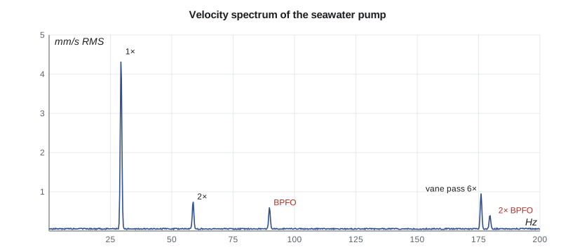
The program stands in for the field data with a synthetic record built from the components Owen measured, plus random noise, and processes it exactly as a collector would: eight seconds at 2,048 samples per second, a Hann window and an FFT with a resolution of 0.125 Hz. The overall level is 4.60 mm/s RMS. The spectrum shows five clear peaks. The largest is 1× at about 4.4 mm/s once corrected for the window (the uncorrected line shows 4.1 because 29.33 Hz falls between lines). The 2× peak is 0.7 mm/s. There is a peak at the outer race defect frequency, 89.8 Hz, at 0.55 mm/s, and another at its second harmonic, 179.6 Hz, at 0.35 mm/s, sitting just 3.6 Hz above the 176 Hz vane-pass peak of 0.9 mm/s. With a coarse resolution of 4 Hz these last two would merge and the bearing harmonic would be missed or blamed on hydraulics.
| Frequency | Source | Typical cause | Seawater pump |
|---|---|---|---|
| 1× | running speed | unbalance, bent shaft, resonance, eccentricity | 4.4 mm/s: dominant |
| 2× | twice running speed | misalignment, looseness | 0.7 mm/s: moderate |
| 0.42 to 0.48× | sub-synchronous | oil whirl (journal bearings) | absent (rolling bearings) |
| BPFO, BPFI, harmonics | bearing defect | race spall or damage | BPFO and 2× BPFO present |
| 6× (vane pass) | hydraulic | impeller-volute gap, off-design flow | 0.9 mm/s: normal for this pump |
| 120 Hz | electrical | motor air gap or supply asymmetry | absent |
| broad band | flow | cavitation, recirculation | low |
Severity: how bad is 4.6 mm/s?
Severity criteria for machinery measured on non-rotating parts are given by the ISO 20816 series, which replaced the long-used ISO 10816 series. They define zones: A, newly commissioned machines; B, acceptable for unrestricted long-term operation; C, unsatisfactory for long-term operation, to be run only until a suitable opportunity for repair; and D, severe enough to cause damage. Zone boundaries depend on the machine type, its size and its support. For small machines, guidance values for velocity of about 0.71, 1.8 and 4.5 mm/s RMS mark the A/B, B/C and C/D boundaries; larger machines and machines on flexible supports are allowed more. Pump-specific parts of the series, and Hydraulic Institute guidance for rotodynamic pumps, give values for different pump types and powers. Tidewater's own acceptance limit for the TP-80 on its test stand is tighter than any of these. The seawater pump, at 4.60 mm/s, is just inside zone D: it should be repaired soon, but it is not about to fly apart. Equally important is the trend: a rise from 1.9 to 4.6 mm/s in three months shows something is changing.
Owen's report quotes the level as 4.6 mm/s RMS, and also as 0.26 in/s peak, the unit the plant's maintenance contractor uses for its alarm settings.
Diagnosis
Owen puts the evidence together. The dominant 1× is similar horizontally and vertically, with a phase difference of about 90° between the two directions and steady phase at constant speed, which points to unbalance (Lesson 6). The pump handles seawater with suspended sand and shell fragments, and its impeller is likely fouled or eroded. The skid's natural frequencies were checked with a bump test (Lesson 3): the first is at 47 Hz, well above running speed, so resonance is ruled out (Lesson 4). The 2× at 0.7 mm/s, with modest axial vibration, suggests some misalignment, perhaps from the skid shifting on the deck. The BPFO peaks, confirmed by envelope analysis with clear harmonics at 89.8, 179.6 and 269.4 Hz, show an outer race defect on the drive-end 6307 bearing; the rising trend matches a spall that is growing. The vane-pass level is the same as it was a year ago and is not a concern.
Worked problem
Remaining life and the repair window
The plant can stop the seawater pump only on a weekend, when the processing line is down, and a spare pump is available for two days. Owen must decide whether the repair can wait three weeks for the scheduled shutdown.
Show solution
- The overall level is 4.6 mm/s and rising about 0.9 mm/s per month; in three weeks it would be about 5.2 mm/s.
- The bearing defect is detectable but not yet at the stage of broad-band noise and many sidebands that marks advanced damage; envelope levels have doubled in a month.
- Risk: a 6307 with a growing outer race spall rarely fails within weeks at this stage, but heat and noise should be checked daily.
Answer: Owen recommends running to the scheduled shutdown with weekly vibration readings and daily temperature checks, and an earlier stop if the overall exceeds 7 mm/s or the bearing temperature rises 10 °C above normal. Condition monitoring is about planning the repair, not just detecting the fault.
Repair and verification
At the shutdown, the maintenance crew, with Owen and Lucie present, finds the impeller coated with marine growth and with its shroud eroded on one side. They clean it, and Tidewater's shop balances it to G6.3; the measured initial unbalance was about 1,400 g·mm, more than four times the limit. The drive-end bearing shows an outer race spall about 4 mm long in the load zone. Both bearings are replaced. The skid has one soft foot, a mounting foot that did not sit flat on its base, which is shimmed, and the coupling is realigned to within 0.05 mm offset. The restart measurement is 1.3 mm/s overall, in zone B, with 1× at 1.0 mm/s, 2× at 0.3 mm/s and no bearing frequencies. Owen sets alarm levels for the monthly route at 2.8 mm/s overall and asks the contractor to add envelope readings on both bearings. He also recommends a strainer upgrade at the intake and a six-monthly impeller inspection, since seawater fouling is the root cause of the unbalance.
Course review: the toolkit
The capstone used nearly every lesson. Harmonic motion and units (Lesson 1) turned the collector's numbers into comparable quantities. Single-degree-of-freedom models and bump tests (Lessons 2 and 3) located the skid's natural frequency and ruled out resonance, the cause of trouble at the Fore River Medical Center, the customer site with rubber pads and the Casco Point Seafoods platform (Lessons 4, 5 and 8). Balancing (Lesson 6) addressed the main fault. Transient analysis (Lesson 7) explained the earlier support crack and shipping damage, torsional modes (Lesson 9) the coupling wear, continuous systems (Lesson 10) the reed frequency and pipe spans, and rotordynamics (Lesson 11) the critical speeds of the multistage rotor. The common thread is Lucie's first instruction: know the natural frequencies, know the forcing frequencies, keep them apart, keep the forces small, and measure to confirm.
Common mistakes
MistakeComparing an overall level measured with a magnet with one measured with a hand probe.
InsteadUse the same sensor, mounting and point each time for trending.
MistakeChoosing a coarse resolution to save time.
InsteadClose components such as 2× BPFO and vane pass need fine resolution.
MistakeReading the uncorrected FFT line as the amplitude.
InsteadCorrect for the window, or sum the power in the lines around the peak.
MistakeJudging only by the absolute level.
InsteadThe trend matters as much; a fast rise demands action even within a zone.
MistakeReplacing a bearing without finding why it failed.
InsteadLook for root causes: unbalance, misalignment, soft foot, lubrication, fouling.
Summary and key terms
- Accelerometers, velocity transducers and proximity probes measure different quantities; mounting limits accelerometer bandwidth.
- An FFT with resolution f_s/N and a Hann window turns a record into a spectrum; resolution must separate close components.
- Bearing defect frequencies BPFO, BPFI, BSF and FTF are non-integer multiples of speed; envelope analysis detects them early.
- Severity zones A to D of the ISO 20816 series judge overall levels; for small machines the C/D boundary is about 4.5 mm/s.
- The seawater pump at 4.6 mm/s had fouling unbalance, a bearing outer race defect and a soft foot; repairs cut it to 1.3 mm/s.
- Vibration engineering is the management of natural frequencies, forcing frequencies and forces, confirmed by measurement.
- Accelerometer
- A transducer whose output is proportional to acceleration.
- Proximity probe
- A non-contacting sensor measuring shaft displacement relative to its bearing.
- Fast Fourier transform
- An efficient algorithm for computing the discrete Fourier spectrum of a sampled signal.
- Frequency resolution
- The spacing of spectral lines, the sample rate divided by the number of samples.
- Aliasing
- The false appearance of high-frequency components at lower frequencies when sampling is too slow.
- Window function
- A taper applied to a record before the FFT to reduce leakage.
- BPFO
- Ball pass frequency of the outer race.
- Envelope analysis
- Demodulation of a high-frequency band to reveal repetitive impacts from bearing defects.
- Severity zone
- A range of vibration levels with a stated meaning for continued operation.
- Soft foot
- A machine foot that does not sit flat, distorting the frame when bolted down.
Practice problems
Work each problem on paper first, then reveal the answer to check.
A collector samples at 2,560 Hz with 4,096 samples. Find the resolution and record length.
Show answer
0.625 Hz; 1.6 s.
A 6205 bearing has 9 balls, d = 7.94 mm, D = 39.0 mm. Find BPFO at 1,780 rpm.
Show answer
4.5 × 29.67 × 0.796 ≈ 106 Hz.
Why should vane-pass and bearing harmonics be separated in the spectrum?
Show answer
They imply different faults: hydraulics versus bearing damage.
A pump runs at 3.2 mm/s steadily for a year. Which zone, for a small machine, and what action?
Show answer
Zone C; plan a repair, investigate the cause, increase monitoring.
In the program, set the BPFO amplitude to 0.05 mm/s. Is it still found as a peak?
Show answer
No: it falls below the 0.2 mm/s threshold and the noise; envelope analysis would be needed.
After repair, the 1× is 1.0 mm/s. What unbalance does that suggest compared with before?
Show answer
About a quarter of the earlier 1× level, consistent with balancing to near G6.3.
Lesson quiz · 5 questions
Score 60% or more to complete this lesson.
Create a free account to save your progress, take quizzes and earn a certificate.