Turbulent boundary layers, transition and separation

The utility's reservoir has a small aluminum workboat that Ray Mendoza's crew uses to tow the maintenance pontoon, inspect the intake tower and take water samples. The outboard motor is near the end of its life, and Ray wants to know whether a smaller electric motor could do the job. The answer depends on the hull's resistance, and at the boat's working speed most of it comes from friction in a turbulent boundary layer. This lesson describes how laminar layers become turbulent, how turbulent layers differ, how to estimate their friction with smooth and rough surfaces, and why turbulence both increases friction drag and delays separation.

Transition to turbulence

A laminar boundary layer on a flat plate does not stay laminar forever. As the Reynolds number based on distance grows, small disturbances in the layer, from free-stream turbulence, surface roughness, vibration or sound, begin to grow instead of dying out. On a smooth plate in a quiet stream, the first unstable waves, called Tollmien-Schlichting waves after the researchers who predicted them, appear at a Reynolds number of about 10⁵. They grow, become three-dimensional, break into turbulent spots, and the spots merge into a fully turbulent layer. The whole process takes place over a transition region.

For engineering calculations, transition on a smooth flat plate is usually taken to occur at a critical Reynolds number:

The real value can range from about 10⁵ in a turbulent free stream or with a rough leading edge to several million in an exceptionally quiet wind tunnel. A favorable pressure gradient delays transition and an adverse one hastens it. On the workboat moving at 2.5 m/s in 10 °C water, transition occurs only about 26 cm behind the bow, so more than 95 percent of the 6 m hull has a turbulent boundary layer. For large vehicles and structures in water or air, the laminar part of the surface is almost always small.

What changes when the layer is turbulent

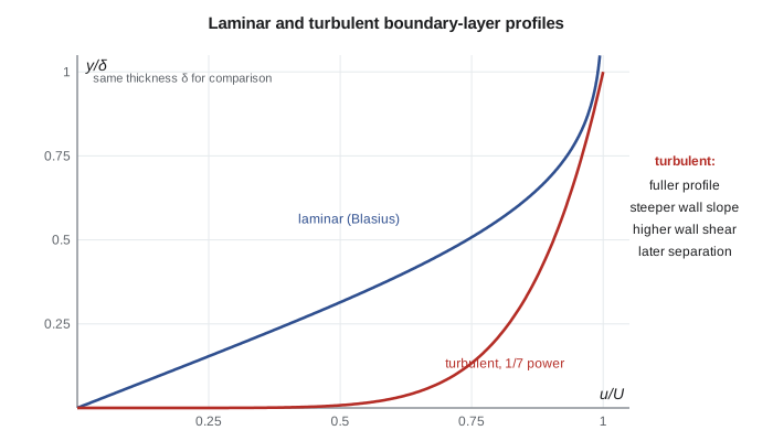
A turbulent boundary layer is full of eddies of many sizes that carry fast fluid toward the wall and slow fluid away from it. That mixing transports momentum far more effectively than molecular viscosity alone. The time-averaged velocity profile is much fuller than the laminar profile: the speed rises very steeply near the wall and then more gently across the outer part of the layer. Three consequences follow. The wall shear stress is much higher, so friction drag is higher. The layer grows faster, roughly as \(x^{4/5}\) instead of \(x^{1/2}\). And because the near-wall fluid is constantly re-energized by mixing, the layer can travel much farther against an adverse pressure gradient before it separates.

A simple and surprisingly accurate description of the mean profile is the one-seventh power law, \(u/U = (y/\delta)^{1/7}\). Combining it with an empirical wall shear law from pipe flow, the momentum-integral method of Lesson 4 gives the classic turbulent flat-plate results, valid for smooth plates from about 5 × 10⁵ to 10⁷:

For a plate with a laminar leading section followed by a turbulent layer, a correction subtracts the turbulent drag that the laminar part did not have; for transition at 5 × 10⁵ it gives \(C_D = 0.074/\text{Re}_L^{1/5} - 1742/\text{Re}_L\). At higher Reynolds numbers, correlations based on the log law are better, such as the Schlichting form \(C_D = 0.455/(\log_{10}\text{Re}_L)^{2.58}\). Naval architects use the ITTC-1957 model-ship correlation line, \(C_F = 0.075/(\log_{10}\text{Re}_L - 2)^2\), as their standard friction line.

Friction on the workboat hull

The workboat's waterline length is 6.0 m and its wetted area is about 14 m². Ray's crew normally runs at 2.5 m/s, about 5 knots, while towing the pontoon. The program computes the hull's friction drag with each correlation, then adds the effect of fouling.

# Turbulent boundary layers: skin friction on the reservoir workboat hull and the log law
import math
rho, nu = 999.7, 1.31e-6          # water at 10 C
U, L, S = 2.5, 6.0, 14.0          # boat speed (m/s), waterline length (m), wetted area (m2)
ReL = U * L / nu
x_tr = 5e5 * nu / U
CD_lam = 1.328 / math.sqrt(ReL)
CD_turb = 0.074 / ReL**0.2
CD_mixed = 0.074 / ReL**0.2 - 1742 / ReL
CD_ittc = 0.075 / (math.log10(ReL) - 2)**2
print(f"Re_L = {ReL:.2e}; transition near x = {x_tr*100:.0f} cm from the bow")
for name, cd in (("all laminar (not real)", CD_lam), ("all turbulent, 1/5 power", CD_turb),
                 ("laminar then turbulent", CD_mixed), ("ITTC-1957 line", CD_ittc)):
    F = cd * 0.5 * rho * U**2 * S
    print(f"  {name:<26} C_D = {cd:.5f}  friction drag {F:6.0f} N  power {F*U/1000:5.2f} kW")
# Boundary-layer thickness at the stern, laminar versus turbulent
print(f"delta at the stern: laminar would be {5.0*L/math.sqrt(ReL)*1000:.0f} mm, turbulent {0.37*L/ReL**0.2*1000:.0f} mm")
# Fouled hull: fully rough plate with roughness height e
for e in (0.0001, 0.001):
    CD_r = (1.89 + 1.62 * math.log10(L / e)) ** -2.5
    print(f"  fully rough, e = {e*1000:.1f} mm: C_D = {CD_r:.5f}, drag {CD_r*0.5*rho*U**2*S:.0f} N")

# Log law near the stern: wall units
cf = 0.0592 / (U * L / nu) ** 0.2
u_tau = U * math.sqrt(cf / 2)
print(f"\nLocal c_f at the stern {cf:.5f}; friction velocity {u_tau:.3f} m/s; viscous length {nu/u_tau*1e6:.1f} micrometers")
for yplus in (1, 5, 30, 100, 1000):
    up = yplus if yplus <= 5 else 2.44 * math.log(yplus) + 5.0
    print(f"  y+ = {yplus:>5}: y = {yplus*nu/u_tau*1000:7.3f} mm, u+ = {up:5.1f}, u = {up*u_tau:.2f} m/s")
# Separation: maximum diffuser half-angle rule of thumb for a pump discharge cone
for half in (3, 5, 8, 12):
    print(f"  conical diffuser half-angle {half} deg:", "attached flow likely" if half <= 5 else "risk of separation and stall")

Re_L = 1.15e+07; transition near x = 26 cm from the bow
  all laminar (not real)     C_D = 0.00039  friction drag     17 N  power  0.04 kW
  all turbulent, 1/5 power   C_D = 0.00287  friction drag    125 N  power  0.31 kW
  laminar then turbulent     C_D = 0.00272  friction drag    119 N  power  0.30 kW
  ITTC-1957 line             C_D = 0.00293  friction drag    128 N  power  0.32 kW
delta at the stern: laminar would be 9 mm, turbulent 86 mm
  fully rough, e = 0.1 mm: C_D = 0.00347, drag 152 N
  fully rough, e = 1.0 mm: C_D = 0.00551, drag 241 N

Local c_f at the stern 0.00229; friction velocity 0.085 m/s; viscous length 15.5 micrometers
  y+ =     1: y =   0.015 mm, u+ =   1.0, u = 0.08 m/s
  y+ =     5: y =   0.077 mm, u+ =   5.0, u = 0.42 m/s
  y+ =    30: y =   0.464 mm, u+ =  13.3, u = 1.13 m/s
  y+ =   100: y =   1.547 mm, u+ =  16.2, u = 1.37 m/s
  y+ =  1000: y =  15.473 mm, u+ =  21.9, u = 1.85 m/s
  conical diffuser half-angle 3 deg: attached flow likely
  conical diffuser half-angle 5 deg: attached flow likely
  conical diffuser half-angle 8 deg: risk of separation and stall
  conical diffuser half-angle 12 deg: risk of separation and stall

The all-laminar estimate, 17 N, is shown only to emphasize how wrong it would be: the real layer is turbulent and the friction is about seven times larger. The turbulent correlations agree within about 8 percent, giving 119 to 128 N of friction drag and 0.30 to 0.32 kW of power to overcome it. The hull also has wave-making and form resistance, and the towed pontoon adds its own drag, so Jun's estimate for the motor allows for a total several times the hull friction. Still, the calculation shows the electric option is realistic: an electric outboard of a few kilowatts can handle the hull itself, and the towing load sets the motor size.

Roughness and fouling

Surface roughness hardly affects a laminar layer but has a large effect on a turbulent one, because the roughness elements poke into the thin, highly sheared region next to the wall. As in pipe flow, three regimes exist. If the roughness height is smaller than the viscous sublayer, the surface is hydraulically smooth. If it is much larger, the surface is fully rough, the drag coefficient becomes independent of Reynolds number, and it depends only on the relative roughness:

Between the two lies a transitional regime. A hull coated with slime and small barnacles or zebra mussels can easily have an equivalent roughness of 0.1 to 1 mm. The program shows that 0.1 mm of roughness raises the hull's friction drag by about a quarter and 1 mm almost doubles it. That is why ships are cleaned and repainted, and why the crew pressure-washes the workboat's hull each spring. The same physics explains why tuberculated old cast-iron mains in MEC-270 carried so much less water than their smooth new replacements.

The inner layer and the law of the wall

Near the wall in any turbulent boundary layer or pipe, the flow depends only on the wall shear stress, the fluid's density and viscosity, and distance from the wall. Dimensional analysis then says that the velocity, scaled by the friction velocity \(u_\tau = \sqrt{\tau_w/\rho}\), is a function of the distance scaled by the viscous length \(\nu/u_\tau\):

Experiments show three regions. In the viscous sublayer, below \(y^+ \approx 5\), \(u^+ = y^+\). In the log-law region, from about \(y^+ = 30\) to a few hundred or more, the velocity follows the logarithmic law of the wall:

where κ ≈ 0.41 is the von Kármán constant. A buffer layer joins the two. The program finds that at the workboat's stern the friction velocity is 0.085 m/s and the viscous length is only 15 micrometers, so the viscous sublayer is less than 0.1 mm thick. This explains why roughness of a tenth of a millimeter makes such a difference: it reaches well beyond the sublayer into the log region. It also explains why CFD models of turbulent flow need either very fine cells at the wall or wall functions based on the log law, a practical point Jun will meet when reviewing the consultant's intake model.

Separation and adverse pressure gradients

Lesson 4 described how an adverse pressure gradient can stop the near-wall fluid and separate a boundary layer. A turbulent layer resists this far better than a laminar one because mixing keeps supplying momentum to the wall region. On a circular cylinder, a laminar layer separates at about 80° from the front; a turbulent layer holds on to about 120°. The difference changes the wake width and the drag dramatically, as Lesson 6 shows.

In internal flow, the most important adverse-gradient device is the diffuser, an expanding passage that converts velocity into pressure. Pump discharge cones, draft tubes below turbines and the expanding sections of venturi meters are all diffusers. If the wall diverges too quickly, the boundary layer separates, the flow detaches from one side and becomes unsteady, and much of the intended pressure recovery is lost. For conical diffusers, the best pressure recovery is usually obtained with a total included angle of about 7 to 10°, a half-angle of roughly 3.5 to 5°. The venturi meter on Northside's transmission main has a 7° outlet cone for this reason, while its inlet cone, where the pressure falls, can be steep.

Controlling transition and separation

Because transition and separation govern drag, engineers manipulate them. Golf balls are dimpled so that their boundary layers become turbulent early and separate late, cutting drag at driving speeds. Vortex generators, small fins on aircraft wings and wind turbine blades, mix high-momentum fluid into the boundary layer and delay stall. Trip wires on wind-tunnel models force transition at the right place so that the model behaves like the full-scale body. In the opposite direction, laminar-flow airfoils, smooth gel coats on racing hulls and polished pipelines aim to keep friction low.

Suction through a porous wall, blowing through slots and moving surfaces are also used to control separation in specialized applications. For water utility equipment, the practical tools are simpler: avoid sudden expansions, give diffusers gentle angles, use long-radius bends and keep straight runs of pipe ahead of flow meters and pump suctions so that the velocity profile is fully developed and free of separated regions when it arrives.

In the United States, the Coast Guard's regulations for recreational-type boats set capacity and maximum horsepower ratings shown on the boat's capacity plate, and an electric outboard must stay within them. The Nebraska utility's fleet policy also requires a check of the boat's rated power before any motor change.