
MEC-370 · Lesson 11 of 12 · 27 min
Pumps: Euler's equation, specific speed and cavitation
MEC-270 treated Pump 2 at Northside as a black box with a head curve, \(H = 78 - 210Q^2\), and an efficiency curve, and found its operating point on the system curve: 0.331 m³/s at 55 m. This lesson opens the box. Jun has received Tidewater Pump Works' preliminary hydraulic design for the replacement pump: a 375 mm impeller with seven backward-curved blades, turning at 1,780 rpm. Hana wants him to check it with the fundamental equation of turbomachinery, to see why the pump has the head it has, how its curve will change on a variable-frequency drive, and whether it will cavitate when the clearwell is low on a hot summer day. These are the questions a utility engineer must be able to ask a pump supplier.
How a centrifugal pump works
Water enters the eye of the impeller axially and turns outward into the passages between the blades. The rotating blades push the water around and outward, increasing both its pressure, through the centrifugal effect and the diffusing action of the widening passages, and its velocity. The water leaves the impeller rim moving fast and swirling, and the volute casing, a spiral passage of growing area, collects it and slows it down, converting much of its kinetic energy into pressure before the discharge nozzle. Double-suction pumps, like the new Pump 2, have impellers that draw water from both sides, which halves the flow through each eye, balances the axial thrust and improves suction performance.
Euler's turbomachine equation
The angular momentum equation from MEC-270, applied to a control volume around the impeller, gives the torque needed to change the swirl of the flow. For steady flow with mass flow ṁ entering at radius r₁ with tangential velocity V_θ1 and leaving at r₂ with V_θ2:
where \(u = \omega r\) is the blade speed. Dividing the power by the weight flow \(\dot m g\) gives the energy added per unit weight, the Euler head:
This is the head an ideal pump, with no losses, would produce. It is valid for any turbomachine: pumps, fans, compressors and, with the sign reversed, turbines. Most pumps are designed with no swirl at the inlet, so the second term vanishes and \(H_E = u_2 V_{\theta 2}/g\). The head depends on the tip speed and on how much swirl the blades put into the water.
Velocity triangles
At the blade exit the absolute velocity of the water V is the vector sum of the blade speed u and the water's velocity relative to the blade W. If the water left exactly along the blade, W would be at the blade angle β₂ measured from the tangent, and the radial component would be set by continuity, \(V_{r2} = Q/(\pi D_2 b_2)\), where b₂ is the impeller width. Then:
This shows the shape of a pump's theoretical head curve. With backward-curved blades, β₂ less than 90°, the head falls linearly as the flow rises. That falling characteristic makes the pump stable on a system curve and prevents its power from rising without limit as the flow increases, which is why almost all centrifugal pumps use backward-curved blades, typically with β₂ between about 15 and 35°.
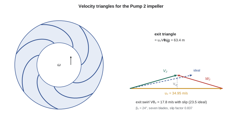
Real impellers have a finite number of blades, and the water between them does not follow the blades exactly. It lags behind the blade direction, an effect called slip, which reduces the exit swirl. Slip is expressed by a slip factor σ, and an empirical formula by Wiesner is widely used for its estimate. With slip, \(V_{\theta 2} = \sigma u_2 - V_{r2}/\tan\beta_2\). Finally, friction, turbulence and recirculation in the impeller and casing dissipate part of the Euler head; the hydraulic efficiency \(\eta_h\) is the ratio of the actual head to the Euler head with slip. Leakage through the wear rings and mechanical friction in bearings and seals lower the overall efficiency further.
# Centrifugal pump: velocity triangles, Euler head, specific speed, affinity laws and NPSH
import math
g, rho = 9.81, 998.0
n = 1780                              # rpm, four-pole motor
Q = 0.331                             # m3/s, duty point from MEC-270
D2, b2, beta2, Z = 0.375, 0.060, math.radians(24), 7    # impeller exit diameter, width, blade angle, blades
D1, b1 = 0.200, 0.100
u2 = math.pi * D2 * n / 60
Vr2 = Q / (math.pi * D2 * b2 * 0.92)  # 0.92 allows for blade blockage
Vt2_ideal = u2 - Vr2 / math.tan(beta2)
sigma = 1 - math.sqrt(math.sin(beta2)) / Z**0.7      # Wiesner slip factor
Vt2 = sigma * u2 - Vr2 / math.tan(beta2)
H_euler_inf = u2 * Vt2_ideal / g      # no inlet swirl
H_euler = u2 * Vt2 / g
eta_h = 0.88
print(f"Tip speed u2 = {u2:.2f} m/s; meridional velocity {Vr2:.2f} m/s")
print(f"Ideal swirl {Vt2_ideal:.2f} m/s -> Euler head {H_euler_inf:.1f} m (infinite blades)")
print(f"Slip factor {sigma:.3f}: swirl {Vt2:.2f} m/s -> Euler head {H_euler:.1f} m; with hydraulic efficiency {eta_h} -> {eta_h*H_euler:.1f} m")
# Inlet triangle: blade angle for shock-free entry with no prerotation
u1 = math.pi * D1 * n / 60
Vm1 = Q / (math.pi * D1 * b1 * 0.90)
beta1 = math.degrees(math.atan(Vm1 / u1))
print(f"Inlet: u1 = {u1:.2f} m/s, Vm1 = {Vm1:.2f} m/s, blade angle {beta1:.1f} deg")

# Specific speed and type number
H = 55.0
Ns_si = n * math.sqrt(Q) / H**0.75
Q_gpm, H_ft = Q * 15850.3, H * 3.28084
Ns_us = n * math.sqrt(Q_gpm) / H_ft**0.75
omega_s = (n * 2 * math.pi / 60) * math.sqrt(Q) / (g * H)**0.75
print(f"\nSpecific speed: {Ns_si:.0f} (rpm, m3/s, m), {Ns_us:,.0f} (rpm, US gpm, ft), dimensionless {omega_s:.2f} rad")

# Affinity laws: running at reduced speed on a variable-frequency drive
H0, a = 78.0, 210.0                   # pump curve H = H0 - a Q^2 at full speed (MEC-270)
dz, ksys = 48.0, 63.9                 # system curve H = dz + k Q^2
for s in (1.00, 0.95, 0.90, 0.85):
    # scaled pump curve: H = s^2 H0 - a Q^2
    Qop = math.sqrt((s**2 * H0 - dz) / (a + ksys)) if s**2 * H0 > dz else 0.0
    Hop = dz + ksys * Qop**2
    print(f"  speed {s:.0%}: operating point {Qop:.3f} m3/s at {Hop:.1f} m")

# NPSH available (from MEC-270) against NPSH required, with margin
patm, pv = 97.4e3, 2.34e3           # vapor pressure at 20 C
z_s, hL_s = 1.5, 0.6
npsha = patm / (rho * g) + z_s - hL_s - pv / (rho * g)
npshr = 7.0                           # NPSH3 from the test, at the duty flow
print(f"\nNPSHA = {npsha:.1f} m, NPSH3 = {npshr} m, margin ratio {npsha/npshr:.2f}")
Nss = n * math.sqrt(Q_gpm) / (npshr * 3.28084)**0.75
print(f"Suction specific speed {Nss:,.0f} (US units); Thoma number {npshr/H:.3f}")
# Summer: warmer water and a low clearwell
npsha_s = patm / (rho * g) + 0.2 - 0.7 - 3.17e3 / (rho * g)
print(f"Low clearwell in summer (25 C): NPSHA = {npsha_s:.1f} m, margin ratio {npsha_s/npshr:.2f}")Tip speed u2 = 34.95 m/s; meridional velocity 5.09 m/s Ideal swirl 23.52 m/s -> Euler head 83.8 m (infinite blades) Slip factor 0.837: swirl 17.81 m/s -> Euler head 63.4 m; with hydraulic efficiency 0.88 -> 55.8 m Inlet: u1 = 18.64 m/s, Vm1 = 5.85 m/s, blade angle 17.4 deg Specific speed: 51 (rpm, m3/s, m), 2,619 (rpm, US gpm, ft), dimensionless 0.96 rad speed 100%: operating point 0.331 m3/s at 55.0 m speed 95%: operating point 0.286 m3/s at 53.2 m speed 90%: operating point 0.235 m3/s at 51.5 m speed 85%: operating point 0.175 m3/s at 49.9 m NPSHA = 10.6 m, NPSH3 = 7.0 m, margin ratio 1.52 Suction specific speed 12,290 (US units); Thoma number 0.127 Low clearwell in summer (25 C): NPSHA = 9.1 m, margin ratio 1.30
The program follows the design step by step. The tip speed is 34.95 m/s and the meridional velocity at the exit is 5.09 m/s. With ideal blade guidance the swirl would be 23.5 m/s and the Euler head 83.8 m. Slip cuts the swirl to 17.8 m/s and the Euler head to 63.4 m; with a hydraulic efficiency of 88 percent the pump develops about 55.8 m at the duty flow, matching the 55 m from the manufacturer's curve within the accuracy of the method. At the inlet, the blade speed at the eye is 18.6 m/s and the axial velocity about 5.9 m/s, so the inlet blades must be set at about 17° to meet the water without incidence. Tidewater's CFD model and the model test of Lesson 2 refine these numbers, but the simple triangles show where the head comes from.
Worked problem
Effect of impeller trimming
Utilities often adjust a pump to its system by trimming the impeller, machining a few percent off its diameter. Estimate the effect of trimming the Pump 2 impeller from 375 to 360 mm on its shutoff head and its best-efficiency flow.
Show solution
- Trimming changes the tip speed and, to a first approximation, scales head with D² and flow with D, because the impeller width and casing stay the same.
- Head ratio \((360/375)^2 = 0.922\): shutoff head \(78 \times 0.922 = 71.9\) m.
- Flow ratio \(360/375 = 0.96\): best-efficiency flow \(0.32 \times 0.96 = 0.307\) m³/s.
Answer: A 4 percent trim lowers the shutoff head by about 6 m and shifts the best-efficiency point down by 4 percent. Trimming is permanent and slightly lowers efficiency, so Hana prefers a variable-frequency drive, which gives the same effect reversibly.
The affinity laws and variable speed
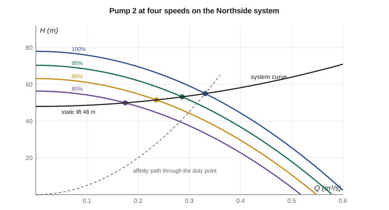
Lesson 2 derived the scaling laws for geometrically similar pumps. For one pump at different speeds, they reduce to the affinity laws: flow proportional to speed, head to speed squared and power to speed cubed, at corresponding points of equal efficiency. Applied to the full-speed curve, they give the curve at any speed. The program finds the operating points on the Northside system curve at 95, 90 and 85 percent speed. Because the system has a large static lift of 48 m, the flow falls much faster than the speed: at 85 percent speed the flow is only 53 percent of the full-speed value. The affinity laws describe the pump, not the system, and a common mistake is to assume that flow on a real system falls in proportion to speed.
Specific speed
Combining the flow and head coefficients to eliminate the diameter gives a group that depends only on the shape of the pump, called the specific speed. It is evaluated at the best-efficiency point:
Unfortunately for students, specific speed is usually quoted in dimensional form, with different units in different countries. With n in rpm, Q in m³/s and H in m, Pump 2's specific speed is about 51. In US practice, with Q in US gallons per minute and H in feet, the same pump has a specific speed of about 2,600. A dimensionless version, with ω in rad/s and gH in J/kg, gives 0.96. Whatever the units, specific speed indicates the impeller type: low values belong to narrow, large-diameter radial impellers for high head and low flow; medium values to mixed-flow impellers; and high values to axial-flow propellers for large flows at low head. It also predicts the best attainable efficiency, which peaks for medium specific speeds and large flows.
| Impeller type | N_s (rpm, m³/s, m) | N_s (rpm, gpm, ft) | Typical use |
|---|---|---|---|
| Radial, narrow | 10 to 30 | 500 to 1,500 | High-head boiler feed, multistage |
| Radial, normal | 30 to 80 | 1,500 to 4,000 | Water supply, Northside Pump 2 |
| Mixed flow | 80 to 160 | 4,000 to 8,000 | Raw-water intakes, irrigation |
| Axial flow (propeller) | 160 to 300 | 8,000 to 15,000 | Storm water, drainage, circulation |
Cavitation
The lowest pressure in a pump occurs just inside the impeller eye, on the suction side of the blades, where the water has been accelerated but has not yet received energy. If the local pressure falls below the vapor pressure, vapor bubbles form. As they are carried into higher-pressure regions they collapse violently, producing noise, vibration, loss of head and pitting damage on the blades. This is cavitation. To prevent it, the pressure at the pump inlet must exceed the vapor pressure by a margin. That margin is the net positive suction head:
for a pump drawing from an open tank whose surface is a height z_s above the pump centerline, with suction loss h_{L,s}. MEC-270 found NPSHA of about 10.6 m at Northside, using Omaha's atmospheric pressure. The pump's required value, NPSHR, is determined by test, conventionally as NPSH3, the suction head at which the total head has dropped by 3 percent because of cavitation. Because cavitation begins well before that point, NPSHA must exceed NPSH3 by a margin. Guidance such as ANSI/HI 9.6.1 recommends margin ratios that depend on the application and the pump's suction energy, commonly in a range of about 1.1 to 2.0 or more for continuous duty.
The program compares Tidewater's NPSH3 of 7.0 m at the duty flow with the available values. In normal conditions the margin ratio is about 1.52. On a hot summer day, with the clearwell drawn down to 0.2 m above the pump centerline, a slightly higher suction loss and water at 25 °C, NPSHA falls to about 9.1 m and the margin ratio to about 1.30. That is acceptable for short periods but low for continuous operation. Jun's recommendation is to raise the minimum clearwell operating level by 0.5 m in the control system, which restores the margin to above 1.3 without changing the pump.
Worked problem
NPSH at higher elevation
Why does a pump at a high-elevation plant have less NPSHA than an identical installation at sea level, and by how much for the Northside conditions?
Show solution
- Atmospheric pressure at Omaha is about 97.4 kPa, compared with 101.3 kPa at sea level: a difference of 3.9 kPa.
- Dividing by ρg: \(3.9\times10^3/(998 \times 9.81) = 0.40\) m.
Answer: The same installation at sea level would have about 0.4 m more NPSHA. At high-elevation sites, and for hot water or volatile liquids, suction conditions often decide the pump's setting, and some pumps must be placed below the water level or fed by a booster.
Suction specific speed and the Thoma number
Replacing the head in the specific speed with NPSH3 gives the suction specific speed, \(N_{ss} = n\sqrt{Q}/\text{NPSH3}^{3/4}\), a measure of how aggressive the impeller's inlet design is. Pump 2's value, in US units, is about 12,300. Impellers with very high suction specific speed achieve low NPSHR at their design flow by using large eyes, but they tend to suffer from suction recirculation, noise and damage at reduced flows. Many users prefer suction specific speeds below a limit of roughly 11,000 to 13,000 in US units for pumps that will operate over a wide flow range. Pump 2 is near that boundary, which is another reason to keep its minimum operating flow, set by the variable-frequency drive, above about 60 percent of best-efficiency flow. The Thoma cavitation number σ = NPSHR/H, here 0.127, is the equivalent ratio used for turbines and in hydropower.
In the United States, pump performance tests are specified to ANSI/HI 14.6, which defines acceptance grades for head, flow, efficiency and power, and NPSH margin guidance comes from ANSI/HI 9.6.1. Platte Bluffs Water's purchase specification calls for a witnessed performance test and an NPSH test at Tidewater's Portland plant before shipment.
Common mistakes
MistakeForgetting slip when estimating head from blade angles.
InsteadApply a slip factor; ideal blade guidance overestimates head by 20 to 30 percent.
MistakeAssuming flow falls in proportion to speed on a real system.
InsteadWith static lift, find the new operating point on the system curve.
MistakeComparing specific speeds in different units.
InsteadCheck whether N_s uses m³/s and m or gpm and ft; the values differ by about 52 times.
MistakeTreating NPSH3 as the onset of cavitation.
InsteadNPSH3 is a 3 percent head drop; cavitation starts earlier, so a margin is needed.
MistakeUsing sea-level atmospheric pressure at an inland plant.
InsteadUse the local station pressure; at Omaha it is about 97.4 kPa.
Summary and key terms
- Euler's equation H_E = (u₂V_θ2 − u₁V_θ1)/g gives the ideal head of any turbomachine from the change in swirl.
- Backward-curved blades give a falling head curve; slip and hydraulic losses reduce the real head below the ideal value.
- For the Pump 2 impeller, the Euler head is 83.8 m ideally, 63.4 m with slip and about 55.8 m with 88 percent hydraulic efficiency.
- Affinity laws scale a pump's curve with speed; on a system with static lift the flow falls faster than the speed.
- Specific speed classifies impellers: Pump 2 is a normal radial design with N_s ≈ 51 (SI) or 2,600 (US units).
- NPSHA must exceed NPSH3 with a margin; at Northside the margin falls from about 1.5 to 1.30 in summer, so the minimum clearwell level is raised.
- Euler's turbomachine equation
- The relation between shaft work and the change in angular momentum of the flow.
- Velocity triangle
- The vector diagram of blade speed, relative velocity and absolute velocity.
- Slip
- The lag of the flow behind the blade direction at an impeller exit.
- Hydraulic efficiency
- The ratio of actual head to Euler head.
- Affinity laws
- Relations scaling a pump's flow, head and power with its speed.
- Specific speed
- A shape parameter n√Q/H^(3/4) evaluated at the best-efficiency point.
- Cavitation
- Formation and collapse of vapor bubbles where pressure falls below the vapor pressure.
- NPSHA
- The net positive suction head available from the installation.
- NPSH3
- The suction head at which the pump's head falls by 3 percent because of cavitation.
- Suction specific speed
- A measure of inlet design, n√Q/NPSH3^(3/4).
Practice problems
Work each problem on paper first, then reveal the answer to check.
An impeller has u₂ = 30 m/s and V_θ2 = 20 m/s with no inlet swirl. Find the Euler head.
Show answer
61.2 m.
Pump 2 runs at 1,600 rpm. Using the affinity laws, find its shutoff head.
Show answer
78 × (1600/1780)² ≈ 63.0 m.
Find the specific speed (SI) of a pump delivering 0.05 m³/s against 80 m at 2,950 rpm.
Show answer
2950 × 0.224/26.7 ≈ 25: a narrow radial impeller.
Convert Pump 2's SI specific speed to US units.
Show answer
About 50.7 × 51.6 ≈ 2,620.
In the program, lower the clearwell to 0 m above the pump centerline in summer. What is the margin ratio?
Show answer
About 1.28.
Why does a pump with high suction specific speed misbehave at low flow?
Show answer
Its large eye promotes suction recirculation, noise and damage away from its design flow.
Lesson quiz · 5 questions
Score 60% or more to complete this lesson.
Create a free account to save your progress, take quizzes and earn a certificate.