
MEC-360 · Lesson 4 of 12 · 23 min
Fatigue with mean stress and variable loading
The rotating-beam test applies fully reversed stress, with a mean of zero. Real parts rarely see that. A spring is preloaded, so its stress never falls to zero. A bolt is tightened before any external load arrives. The TP-80 shaft sees fully reversed bending from the impeller load, but its torque is nearly steady, which adds a mean shear stress. And no machine runs at one load forever: the TP-80 runs at its best efficiency point most of the time, but customers also throttle it far back on its curve, start and stop it, and occasionally let it run dry. This lesson extends the fatigue model to mean stresses and to loads that change from cycle to cycle.
Describing a fluctuating stress
A stress that cycles between a maximum and a minimum can be described by its alternating component and its mean component:
Other common terms are the stress range \(\Delta\sigma = 2\sigma_a\), the stress ratio \(R = \sigma_{\min}/\sigma_{\max}\) and the amplitude ratio \(A = \sigma_a/\sigma_m\). Fully reversed stress has R = −1; a stress that rises from zero and returns, such as a bolt in a pressurized flange, has R = 0 and is called repeated or pulsating. Stress concentration factors apply to both components; the usual practice for ductile materials is to apply \(K_f\) to both, provided the peak stress stays below yield.
Experiments show that a tensile mean stress reduces the alternating stress a part can survive, while a compressive mean stress has little effect or even helps. That is why compressive residual stresses from shot peening improve fatigue life: they lower the effective mean stress at the surface where cracks start.
The Haigh diagram and its failure lines
Mean stress effects are shown on a plot of alternating stress against mean stress, often called a Haigh diagram or a modified Goodman diagram. The point \((0, S_e)\) on the vertical axis is fully reversed loading at the endurance limit; the point \((S_{ut}, 0)\) on the horizontal axis is static failure. Test data for steels fall between a straight line and a parabola joining these points. Several criteria are in use:
| Criterion | Failure line | Factor of safety n |
|---|---|---|
| Goodman | \(\sigma_a/S_e + \sigma_m/S_{ut} = 1\) | \(1/n = \sigma_a/S_e + \sigma_m/S_{ut}\) |
| Soderberg | \(\sigma_a/S_e + \sigma_m/S_y = 1\) | \(1/n = \sigma_a/S_e + \sigma_m/S_y\) |
| Gerber | \(\sigma_a/S_e + (\sigma_m/S_{ut})^2 = 1\) | Quadratic in n; solved in the program |
| ASME-elliptic | \((\sigma_a/S_e)^2 + (\sigma_m/S_y)^2 = 1\) | \(1/n^2 = (\sigma_a/S_e)^2 + (\sigma_m/S_y)^2\) |
| Langer (first-cycle yield) | \(\sigma_a + \sigma_m = S_y\) | \(n = S_y/(\sigma_a + \sigma_m)\) |
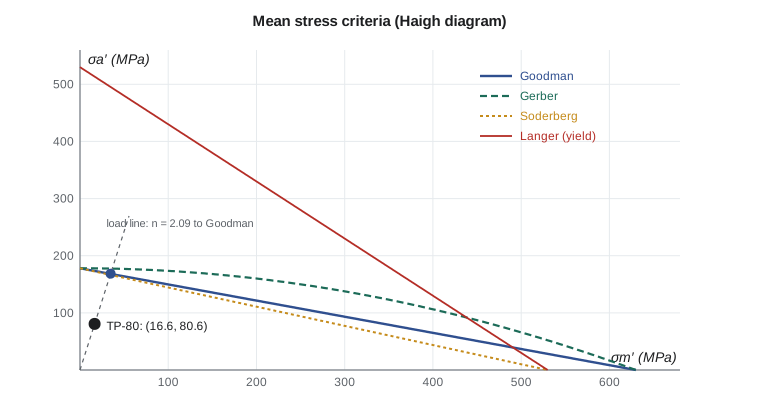
Goodman is the most widely used: it is conservative, linear and simple. Soderberg is more conservative and is rarely used now except where yielding must be strictly avoided. Gerber and ASME-elliptic fit test data for ductile steels more closely and are used when a less conservative estimate is justified, for example in shaft design to the ASME approach. With any of the fatigue criteria, a separate check for first-cycle yielding, the Langer line, is needed when mean stresses are large, because the Gerber and ASME curves extend above the yield line near the mean stress axis.
Combined stresses: equivalent alternating and mean stresses
When a part sees fluctuating bending and fluctuating torsion together, the distortion energy theory is applied separately to the alternating and mean components to form equivalent stresses:
These are then used in the chosen criterion with the corrected endurance limit \(S_e\) for bending. For the TP-80 shaft, rotating bending gives a purely alternating normal stress and the steady motor torque gives a purely mean shear stress, so \(\sigma_a' = K_f\sigma_a\) and \(\sigma_m' = \sqrt3 K_{fs}\tau_m\).
# Fluctuating stress at the TP-80 shoulder: Goodman, Gerber, ASME-elliptic, Soderberg and Miner's rule
import math
Sut, Sy, Se = 630.0, 530.0, 178.0          # MPa (Se from Lesson 3)
d, M, T = 0.035, 216.0, 59.7
Kf, Kfs = 1.57, 1.35                       # fatigue concentration factors (bending, torsion)
sa = Kf * 32 * M / (math.pi * d**3) / 1e6        # rotating bending -> fully reversed
tm = Kfs * 16 * T / (math.pi * d**3) / 1e6       # steady torque -> mean shear
sa_vm, sm_vm = sa, math.sqrt(3) * tm
print(f"alternating sigma_a' = {sa_vm:.1f} MPa, mean sigma_m' = {sm_vm:.1f} MPa")
n_good = 1 / (sa_vm / Se + sm_vm / Sut)
n_sod = 1 / (sa_vm / Se + sm_vm / Sy)
n_ger = 0.5 * (Sut / sm_vm)**2 * (sa_vm / Se) * (-1 + math.sqrt(1 + (2 * sm_vm * Se / (Sut * sa_vm))**2))
n_asme = 1 / math.sqrt((sa_vm / Se)**2 + (sm_vm / Sy)**2)
n_y = Sy / (sa_vm + sm_vm)
for name, n in (("Goodman", n_good), ("Soderberg", n_sod), ("Gerber", n_ger), ("ASME-elliptic", n_asme), ("first-cycle yield (Langer)", n_y)):
    print(f"  {name:27s} n = {n:.2f}")

# Variable amplitude: a year of duty at the plant, with Miner's rule
a, b = 1653.0, -0.1614                     # S-N line from Lesson 3 (MPa, exponent)
duty = [  # (description, alternating stress MPa, cycles per year)
    ("normal flow",              80,  1760 * 60 * 6000),
    ("flow far left of BEP",    150,  1760 * 60 * 400),
    ("starts with hammer",      320,  2 * 365 * 3),
    ("dry-run trips",           240,  12 * 2000),
]
D = 0.0
for name, s, n in duty:
    N = (s / a) ** (1 / b) if s > Se else float('inf')
    frac = n / N if N != float('inf') else 0.0
    D += frac
    print(f"{name:21s} {s:4d} MPa  n = {n:>12,}  N = {('infinite' if N == float('inf') else f'{N:,.0f}'):>12}  n/N = {frac:.4f}")
print(f"Miner damage per year D = {D:.4f} -> predicted life about {1/D:.1f} years")alternating sigma_a' = 80.6 MPa, mean sigma_m' = 16.6 MPa Goodman n = 2.09 Soderberg n = 2.07 Gerber n = 2.20 ASME-elliptic n = 2.20 first-cycle yield (Langer) n = 5.46 normal flow 80 MPa n = 633,600,000 N = infinite n/N = 0.0000 flow far left of BEP 150 MPa n = 42,240,000 N = infinite n/N = 0.0000 starts with hammer 320 MPa n = 2,190 N = 26,203 n/N = 0.0836 dry-run trips 240 MPa n = 24,000 N = 155,758 n/N = 0.1541 Miner damage per year D = 0.2377 -> predicted life about 4.2 years
Worked problem
Fatigue factor of safety for the TP-80 shoulder
With \(K_f = 1.57\), \(K_{fs} = 1.35\), M = 216 N·m, T = 59.7 N·m, d = 35 mm, \(S_e = 178\) MPa and \(S_{ut} = 630\) MPa, find the Goodman factor of safety.
Show solution
- \[\sigma_a' = 1.57\frac{32(216)}{\pi(0.035)^3} = 80.6\ \text{MPa}, \qquad \sigma_m' = \sqrt3 \times 1.35 \frac{16(59.7)}{\pi(0.035)^3} = 16.6\ \text{MPa}\]
- \[\frac{1}{n} = \frac{80.6}{178} + \frac{16.6}{630} = 0.453 + 0.026 = 0.479, \qquad n = 2.09\]
Answer: The Goodman factor of 2.09 meets Farah's design factor of 2. The Gerber and ASME-elliptic criteria give 2.20, and first-cycle yield is not a concern at 5.5. Because the torque contributes only a small mean stress, the result is close to the fully reversed value \(S_e/\sigma_a' = 2.21\). Fatigue, not static strength, governs the shaft size.
Variable amplitude loading and Miner's rule
When the stress amplitude changes from cycle to cycle, the simplest model of damage is the linear damage rule proposed by Palmgren and Miner. Each cycle at stress amplitude \(\sigma_i\) uses up a fraction \(1/N_i\) of the life, where \(N_i\) is the life at that stress from the S-N curve. Failure is predicted when the fractions add to one:
For the TP-80, Farah estimates a year of service at a typical water utility: 6,000 hours at the normal duty with an alternating stress of 80 MPa; 400 hours throttled far left of the best efficiency point, where hydraulic radial loads rise and the stress reaches about 150 MPa; two starts a day with a pressure surge raising the stress briefly to about 320 MPa for three cycles; and a monthly test trip of the dry-run protection, during which rubbing at the wear rings raises the stress to about 240 MPa for about 2,000 cycles. Stresses at or below the endurance limit contribute no damage in the basic rule. The surges and dry-run events do.
Worked problem
Damage from the yearly duty
Use the S-N line from Lesson 3 (a = 1653 MPa, b = −0.1614) to find the damage per year.
Show solution
- Starts: \(N = (320/1653)^{-1/0.1614} = 26\,200\); n = 2,190 per year; \(n/N = 0.084\).
- Dry-run trips: \(N = (240/1653)^{-1/0.1614} = 156\,000\); n = 24,000; \(n/N = 0.154\).
- Normal and throttled running: below \(S_e\), no damage counted.
- \(D = 0.238\) per year, so the predicted life is about 4.2 years.
Answer: This is an important result. The shaft that passes its fatigue check with n = 2.1 at the normal duty could fail in about four years because of a few thousand high-stress cycles a year. The design response is not to make the shaft much bigger but to remove the causes: Tidewater recommends a soft starter or check-valve damping to the customer to control the surge, and moves the dry-run test to a lower-speed check. Without the surge, the damage falls to 0.154 per year; without both, the shaft has infinite life by this model.
Miner's rule is easy to use but has known weaknesses. The order of loading matters in reality: high stresses first, followed by low stresses, are more damaging than the reverse, because a crack started by the high stresses can then grow under stresses that would never have started one. Tests show that failure can occur with D anywhere from about 0.3 to 3. In addition, stresses below the original endurance limit can cause damage once a crack exists. Modified approaches, such as extending the S-N line below the knee with a shallower slope (the Haibach approach), are used in standards for welded structures and some machine elements. A cautious designer uses a damage limit below 1, such as 0.3 to 0.5 for critical parts, or tests the part under a representative load spectrum.
Counting cycles
When the load history is measured rather than estimated, as with strain gauges on a shaft in service, the cycles must be counted before Miner's rule can be applied. The standard method is rainflow counting, which pairs peaks and valleys in a way that matches the closed stress-strain loops seen in the material. Each counted cycle has a range and a mean; mean stress effects are included by converting each cycle to an equivalent fully reversed amplitude with the Goodman or another criterion. Software for rainflow counting is widely available, and ASTM E1049 describes the procedure.
In US units the TP-80 shoulder stresses are 11.7 ksi alternating and 2.4 ksi mean, against \(S_e = 25.8\) ksi and \(S_{ut} = 91.4\) ksi; the Goodman factor is the same 2.09. Variable-speed drives are increasingly common in US water systems, partly because of utility incentive programs and partly because they soften starts and stops, which, as the Miner's rule example shows, can matter more for shaft life than the steady running load.
Common mistakes
MistakeIgnoring the mean stress from a steady torque or preload.
InsteadCombine alternating and mean components and use a mean stress criterion.
MistakeUsing the Gerber or ASME-elliptic line without a yield check.
InsteadAlso check the Langer line, σ_a + σ_m ≤ S_y.
MistakeTreating Miner's rule as exact.
InsteadFailure can occur at damage sums well below 1; use a lower limit or test.
MistakeCounting no damage from stresses below the endurance limit after large overloads.
InsteadOverloads can start cracks that then grow at lower stresses; consider extending the S-N line.
MistakeDesigning a bigger part to absorb an avoidable overload.
InsteadRemove or limit the cause, such as pressure surges, when possible.
Summary and key terms
- A fluctuating stress has an alternating component σ_a and a mean component σ_m; tensile mean stress reduces fatigue strength.
- Goodman, Soderberg, Gerber and ASME-elliptic criteria relate σ_a and σ_m to S_e and S_ut or S_y; Goodman is the usual conservative choice.
- Combined stresses use von Mises equivalents for the alternating and mean components separately.
- The TP-80 shoulder has a Goodman factor of 2.09, meeting the design factor of 2.
- Miner's rule sums n_i/N_i; for the TP-80, starts with pressure surges and dry-run trips give a predicted life of only about four years.
- Miner's rule ignores load order and scatter; use damage limits below 1 for critical parts.
- Alternating stress
- Half the range of a fluctuating stress.
- Mean stress
- The average of the maximum and minimum stresses in a cycle.
- Stress ratio
- R = σ_min/σ_max.
- Haigh diagram
- A plot of alternating against mean stress showing fatigue failure lines.
- Goodman criterion
- A straight failure line joining S_e on the alternating axis to S_ut on the mean axis.
- Langer line
- The first-cycle yield line σ_a + σ_m = S_y.
- Miner's rule
- The linear damage rule: failure when the sum of cycle ratios n_i/N_i reaches one.
- Rainflow counting
- A method for counting cycles in an irregular load history.
- Load spectrum
- The distribution of load or stress levels and their numbers of cycles over a period of service.
Practice problems
Work each problem on paper first, then reveal the answer to check.
A stress varies from −40 to 160 MPa. Find σ_a, σ_m and R.
Show answer
σ_a = 100 MPa, σ_m = 60 MPa, R = −0.25.
For σ_a = 100 MPa, σ_m = 60 MPa, S_e = 200 MPa and S_ut = 700 MPa, find the Goodman factor of safety.
Show answer
n = 1.70.
For the same stresses with S_y = 500 MPa, find the ASME-elliptic factor.
Show answer
n = 1.94.
In the program, remove the starts with surge from the duty list. What is the predicted life?
Show answer
About 6.5 years.
A part sees 10⁴ cycles at a stress whose life is 5 × 10⁴, then 2 × 10⁵ cycles at a stress whose life is 10⁶. Find D.
Show answer
D = 0.4.
Why does a compressive residual stress at the surface improve fatigue life?
Show answer
It lowers the effective mean stress where cracks start.
Lesson quiz · 5 questions
Score 60% or more to complete this lesson.
Create a free account to save your progress, take quizzes and earn a certificate.