
MEC-360 · Lesson 3 of 12 · 21 min
Fatigue fundamentals: S-N curves and the endurance limit
The TP-80 shaft turns 1,760 times a minute. Each turn carries every point on its surface from the tension side of the bend to the compression side and back, so a point at the shoulder fillet sees a full cycle of reversed stress every 34 milliseconds. In a year of continuous running that is more than 900 million cycles. A stress that would do no harm if applied once can, repeated that many times, start a crack that grows until the shaft breaks. Most mechanical failures of rotating machinery are fatigue failures, and they happen at stresses well below the yield strength, with no visible warning before the final fracture. This lesson explains how fatigue strength is measured and how a laboratory value is corrected for a real part.
How fatigue failures happen
Fatigue failure has three stages. A crack initiates at a point of high local stress, almost always at the surface: a fillet, a keyway corner, a machining mark, a corrosion pit or an inclusion just below the surface. The crack then propagates slowly with each cycle, advancing perhaps a fraction of a micrometer per cycle, and leaves beach marks on the fracture surface where it paused or the load changed. Finally, when the remaining section is too small to carry the load, it breaks suddenly. The fracture surface of a fatigued shaft shows a smooth, often curved zone where the crack grew and a rough zone where the final fracture occurred. Marco Rossi, Tidewater's quality inspector, keeps a shelf of broken shafts returned from the field, and the pattern is the same on nearly all of them: a smooth crescent starting at a keyway or a shoulder, and a small rough area where the shaft finally let go.
Because initiation depends on surface details, fatigue strength depends strongly on surface finish, size, the type of loading and the environment, much more than static strength does. Because propagation takes many cycles, regular inspection can sometimes find cracks before they cause failure, which is the basis of inspection programs for aircraft and large machinery.
The rotating-beam test and the S-N diagram
The classic fatigue test, developed by R. R. Moore, spins a small polished specimen while a dead weight bends it, so every point on the surface sees fully reversed bending stress. Specimens are tested at several stress levels and the number of cycles to failure is recorded. Plotted on log-log axes, stress amplitude against cycles to failure gives the S-N diagram. For steels the curve has three regions. Below about 1,000 cycles is low-cycle fatigue, where stresses are near the ultimate strength and plastic strain dominates. Between about 10³ and 10⁶ cycles is high-cycle fatigue with finite life, where the curve is nearly a straight line on log-log axes. Beyond about 10⁶ cycles, most steels show a knee and the curve becomes nearly flat: below this stress, the endurance limit, the specimen does not fail at all in practical test durations.
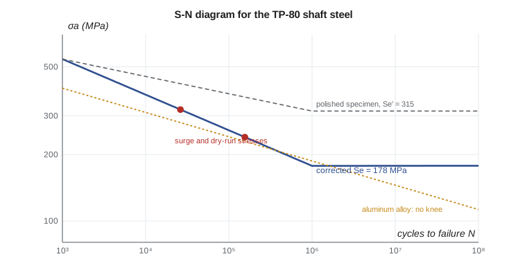
Not every material has an endurance limit. Aluminum alloys, copper alloys and most nonferrous metals keep losing strength as cycles increase, so they are rated by a fatigue strength at a stated life, often \(5 \times 10^8\) cycles. Even for steel, the endurance limit can disappear in a corrosive environment, at high temperature, or after occasional large overloads, and very-high-cycle testing has found failures beyond \(10^9\) cycles that start at internal inclusions. For design purposes, the endurance limit of steel is still a useful and widely used concept, but it should be treated as a model, not a guarantee.
Estimating the endurance limit
Fatigue tests are expensive, so designers often estimate the endurance limit of a polished specimen from the ultimate strength. For steels, test data show the endurance limit is roughly half the ultimate strength up to an ultimate of about 1,400 MPa (200 ksi), after which it levels off:
The prime marks a value for the ideal laboratory specimen. The scatter in the data is large; the ratio ranges from about 0.4 to 0.6, which is one reason for testing real parts when the stakes are high.
Marin factors: from specimen to part
A real shaft differs from the test specimen in surface finish, size, loading, temperature and the reliability required. Following an approach proposed by Joseph Marin, each difference is represented by a factor that multiplies the specimen value:
| Factor | Accounts for | Typical form or value |
|---|---|---|
| \(k_a\) | Surface condition | \(a\,S_{ut}^{\,b}\); machined or cold-drawn a = 4.51, b = −0.265 (MPa) |
| \(k_b\) | Size (bending, torsion) | \(1.24\,d^{-0.107}\) for 2.79 ≤ d ≤ 51 mm; 1 for axial loading |
| \(k_c\) | Type of loading | 1 bending; 0.85 axial; 0.59 torsion alone |
| \(k_d\) | Temperature | 1 near room temperature; lower above about 250 °C |
| \(k_e\) | Reliability | 1 at 50 %; 0.897 at 90 %; 0.814 at 99 %; 0.753 at 99.9 % |
| \(k_f\) | Other effects | Corrosion, plating, fretting, residual stress; often 1 with judgment |
The surface factor is the largest correction for most parts. A polished specimen has almost no initiation sites; a machined surface has tool marks; a hot-rolled or forged surface has scale and decarburization, which can halve the fatigue strength of a high-strength steel. Stronger steels are more sensitive to surface condition, which is why the exponent b is negative: the factor falls as the ultimate strength rises. The size factor reflects the greater chance that a larger part contains a weak spot in its highly stressed volume. The reliability factor shifts the mean strength down by a number of standard deviations, assuming about 8 percent scatter.
For the TP-80 shaft, made from cold-drawn 1045 with an ultimate strength of 630 MPa, machined at the bearing seat, 35 mm in diameter, in rotating bending at room temperature, and designed for 99 percent reliability, the program below gives \(k_a = 0.817\), \(k_b = 0.848\) and \(k_e = 0.814\), and a corrected endurance limit of 178 MPa, little more than half the specimen value of 315 MPa.
# Fatigue strength of the TP-80 shaft: Marin factors, S-N line and notch sensitivity
import math
Sut = 630.0                                   # MPa, cold-drawn 1045 (typical)
Se_prime = 0.5 * Sut if Sut <= 1400 else 700.0
ka = 4.51 * Sut ** -0.265                      # machined or cold-drawn surface
d = 35.0
kb = 1.24 * d ** -0.107 if d <= 51 else 1.51 * d ** -0.157   # rotating bending
kc, kd, ke = 1.0, 1.0, 0.814                   # bending, room temperature, 99 % reliability
Se = ka * kb * kc * kd * ke * Se_prime
print(f"Se' = {Se_prime:.0f} MPa; ka = {ka:.3f}, kb = {kb:.3f}, ke = {ke}")
print(f"corrected endurance limit Se = {Se:.0f} MPa")

# S-N line between 10^3 and 10^6 cycles: S = a N^b
f = 0.86                                      # fatigue strength fraction at 10^3 cycles for Sut near 630 MPa
a = (f * Sut) ** 2 / Se
b = -math.log10(f * Sut / Se) / 3
print(f"S-N line: a = {a:.0f} MPa, b = {b:.4f}")
for sa in (450, 350, 300, 260):
    N = (sa / a) ** (1 / b) if sa > Se else float('inf')
    print(f"  fully reversed stress {sa} MPa -> life {'infinite' if N == float('inf') else f'{N:,.0f} cycles'}")

# Notch sensitivity (Neuber) at the bearing shoulder fillet, r = 2.5 mm
r = 2.5
sqrt_a_b = 0.246 - 3.08e-3 * (Sut/6.895) + 1.51e-5 * (Sut/6.895)**2 - 2.67e-8 * (Sut/6.895)**3   # sqrt(in), bending
sqrt_a_mm = sqrt_a_b * math.sqrt(25.4)
q = 1 / (1 + sqrt_a_mm / math.sqrt(r))
Kt = 1.7
Kf = 1 + q * (Kt - 1)
print(f"\nNeuber constant {sqrt_a_mm:.3f} sqrt(mm), q = {q:.2f}, Kf = {Kf:.2f} (Kt = {Kt})")
hours = 1e6 / (1760 * 60)
print(f"at 1,760 rpm, 10^6 cycles pass in {hours:.1f} hours; 10^9 cycles in {hours*1000/24/365:.1f} years of continuous running")Se' = 315 MPa; ka = 0.817, kb = 0.848, ke = 0.814 corrected endurance limit Se = 178 MPa S-N line: a = 1653 MPa, b = -0.1614 fully reversed stress 450 MPa -> life 3,158 cycles fully reversed stress 350 MPa -> life 14,977 cycles fully reversed stress 300 MPa -> life 38,912 cycles fully reversed stress 260 MPa -> life 94,412 cycles Neuber constant 0.354 sqrt(mm), q = 0.82, Kf = 1.57 (Kt = 1.7) at 1,760 rpm, 10^6 cycles pass in 9.5 hours; 10^9 cycles in 1.1 years of continuous running
Finite life: the S-N line
Between 10³ and 10⁶ cycles the S-N curve for steel is approximated by a straight line on log-log axes, \(S_f = a N^b\). The line passes through \(f S_{ut}\) at 10³ cycles and \(S_e\) at 10⁶ cycles, where f is a fatigue strength fraction that depends on the ultimate strength (about 0.9 for steels near 500 MPa, falling to about 0.8 near 1,400 MPa). Then
Worked problem
Life of the shaft at a high stress
During a water hammer event at a customer's plant, the TP-80 shoulder sees a fully reversed stress amplitude of 300 MPa. With f = 0.86, \(S_{ut} = 630\) MPa and \(S_e = 178\) MPa, how many such cycles can it survive?
Show solution
- \[a = \frac{(0.86 \times 630)^2}{178} = 1653\ \text{MPa}, \qquad b = -\frac{1}{3}\log\frac{541.8}{178} = -0.1614\]
- \[N = \Big(\frac{300}{1653}\Big)^{1/(-0.1614)} \approx 39\,000\ \text{cycles}\]
Answer: At 1,760 rpm, 39,000 cycles pass in about 22 minutes. A shaft that sees such a stress for even a short time each start will fail quickly. In practice a water hammer event lasts only a few cycles, but the result shows how fast life falls as stress rises: a 15 percent increase in stress from 260 to 300 MPa cuts the life by more than half. Lesson 4 shows how to add up damage from a mixture of such events.
Notch sensitivity and the fatigue stress concentration factor
In fatigue, stress concentration matters, but not always by the full theoretical factor \(K_t\). Very sharp notches in soft materials have less effect than elasticity predicts, because the high stress acts on a very small volume. The effective factor is the fatigue stress concentration factor \(K_f\), related to \(K_t\) by the notch sensitivity q:
where r is the notch radius and \(\sqrt a\) is the Neuber constant, a material property that falls as strength rises. A value of q = 0 means the material ignores the notch; q = 1 means full sensitivity. High-strength steels are close to 1, which is why a hardened shaft with a sharp keyway can be weaker in fatigue than a softer shaft with the same keyway. For the TP-80 shoulder, with a 2.5 mm radius in 630 MPa steel, the program gives q = 0.82 and \(K_f = 1.57\), compared with \(K_t = 1.7\). In torsion the Neuber constant is smaller, and the program's value carries through to \(K_{fs} \approx 1.35\) used in later lessons.
The usual practice is to apply \(K_f\) to the stress and compare with the unnotched endurance limit \(S_e\), rather than reducing the strength. The two are equivalent for fully reversed stress, but applying \(K_f\) to the stress keeps the bookkeeping clear when mean stresses are added in the next lesson.
Designing against fatigue
Because fatigue starts at surfaces and discontinuities, many of the best defenses are in detailing rather than size. Generous fillets, a keyway with a sled-runner end instead of an end-milled pocket, threads with rolled roots, and keyways and holes moved away from the highest-stress sections all reduce \(K_f\). Surface treatments that leave compressive residual stress, such as shot peening, cold rolling of fillets and case hardening, delay crack initiation and can raise the endurance limit substantially. Corrosion is a strong enemy of fatigue strength, and a shaft wetted by process liquid may need a sleeve or a stainless steel.
In US units, the TP-80 shaft steel has \(S_{ut} \approx 91\) ksi, a specimen endurance limit of about 45.7 ksi and a corrected limit of about 25.8 ksi. In those units the surface factor is \(a S_{ut}^b\) with a = 2.70 and b = −0.265 for a machined surface, and the size factor is \(0.879 d^{-0.107}\) with d in inches, for 0.11 to 2 in. These give the same results as the SI forms.
Common mistakes
MistakeUsing the specimen endurance limit S_e′ for a real part.
InsteadApply the Marin factors; for a machined shaft the corrected value can be half of S_e′.
MistakeAssuming every material has an endurance limit.
InsteadAluminum and copper alloys do not; use a fatigue strength at a stated life.
MistakeApplying K_t in full to a soft steel with a sharp notch.
InsteadUse the notch sensitivity to find K_f.
MistakeUsing the bending size factor for axial loading.
InsteadFor axial loading, k_b = 1 and k_c = 0.85.
MistakeForgetting that a corrosive environment can remove the endurance limit.
InsteadUse fatigue data measured in the service environment.
Summary and key terms
- Fatigue cracks initiate at surfaces and stress raisers, grow slowly with each cycle, and end in sudden fracture.
- The S-N diagram for steel is a straight line on log-log axes between 10³ and 10⁶ cycles, with an endurance limit beyond.
- For steel, S_e′ ≈ 0.5 S_ut up to 1,400 MPa; the Marin factors for surface, size, loading, temperature and reliability correct it for a real part.
- The TP-80 shaft's corrected endurance limit is 178 MPa, about 57 percent of the specimen value.
- Finite life follows N = (σ_a/a)^(1/b); small increases in stress cut life sharply.
- Notch sensitivity gives K_f = 1 + q(K_t − 1); at the TP-80 shoulder K_f = 1.57.
- Fatigue
- Failure under repeated stress at levels below the static strength.
- Endurance limit
- The fully reversed stress below which a steel specimen does not fail in practical lives.
- S-N diagram
- A plot of stress amplitude against cycles to failure.
- Rotating-beam test
- A fatigue test in which a spinning specimen is loaded in bending so each surface point sees fully reversed stress.
- Marin factors
- Multipliers that correct the specimen endurance limit for surface, size, loading, temperature, reliability and other effects.
- Notch sensitivity
- The fraction of the theoretical stress concentration that is effective in fatigue.
- Fatigue stress concentration factor
- K_f, the effective stress concentration in fatigue.
- Beach marks
- Curved lines on a fatigue fracture surface showing successive positions of the crack front.
- Shot peening
- A surface treatment that leaves compressive residual stress and raises fatigue strength.
Practice problems
Work each problem on paper first, then reveal the answer to check.
Find S_e′ and k_a for a machined steel with S_ut = 800 MPa.
Show answer
S_e′ = 400 MPa; k_a = 0.766.
Find k_b for a 25 mm shaft in rotating bending.
Show answer
0.879.
Using a = 1653 MPa and b = −0.1614, find the life at 350 MPa.
Show answer
About 15,000 cycles.
A notch has K_t = 2.0 and q = 0.85. Find K_f.
Show answer
1.85.
In the program, change the reliability to 99.9 percent (k_e = 0.753). Find the new S_e.
Show answer
About 165 MPa.
Why are high-strength steels more sensitive to surface finish?
Show answer
Their higher strength depends on a flaw-free surface, so tool marks and scale cut their fatigue strength more.
Lesson quiz · 5 questions
Score 60% or more to complete this lesson.
Create a free account to save your progress, take quizzes and earn a certificate.