Functions of a complex variable and mappings

A function of a complex variable assigns to each \(z\) in some set a complex number \(f(z)\). Because both the input and the output are points in a plane, we cannot draw the graph of such a function the way we graph \(y = f(x)\); the graph would live in four real dimensions. Instead we picture a complex function as a mapping: it moves the points of one plane, the \(z\)-plane, to points of another, the \(w\)-plane. This lesson builds the vocabulary of sets in the plane, splits complex functions into real and imaginary parts, and studies the basic mappings, linear maps, powers, inversion and the exponential, that we will use for the rest of the course.

Sets in the complex plane

Complex analysis needs a few words to describe the sets on which functions are defined. The open disk of radius \(r > 0\) about \(z_0\) is \(D(z_0, r) = \{z : |z - z_0| < r\}\); a punctured disk leaves out the center point. A set \(U\) is open if every point of \(U\) is the center of some open disk contained in \(U\). Open disks, open half-planes such as \(\operatorname{Im} z > 0\), and the whole plane are open; a closed disk \(|z - z_0| \le r\) is not, because no disk about a boundary point stays inside it.

A set is connected, in the sense we need, if any two of its points can be joined by a path made of finitely many line segments lying in the set. An open connected set is called a domain or region. Domains are the natural places to define analytic functions: openness lets us take limits from every direction, and connectedness rules out a set made of separate islands on which a function could behave independently. The annulus \(1 < |z| < 2\) is a domain; the union of two disjoint disks is open but not a domain.

A set is bounded if it lies inside some disk about 0. A domain is simply connected if every closed path in it can be shrunk to a point without leaving the domain; informally, it has no holes. Disks and half-planes are simply connected; the annulus and the punctured plane \(\mathbb{C} \setminus \{0\}\) are not. This distinction will matter enormously in lesson 7.

Real and imaginary parts

Writing \(z = x + iy\) and \(f(z) = w = u + iv\), every complex function is a pair of real functions of two real variables:

\[f(x + iy) = u(x, y) + i\,v(x, y).\]

For \(f(z) = z^2\) we get \((x + iy)^2 = x^2 - y^2 + 2ixy\), so \(u = x^2 - y^2\) and \(v = 2xy\). For \(f(z) = \frac{1}{z}\) we get \(\frac{\bar{z}}{|z|^2} = \frac{x - iy}{x^2 + y^2}\), so \(u = \frac{x}{x^2 + y^2}\) and \(v = \frac{-y}{x^2 + y^2}\). For \(f(z) = \bar{z}\), \(u = x\) and \(v = -y\).

So in one sense a complex function is nothing new: it is a map from \(\mathbb{R}^2\) to \(\mathbb{R}^2\) of the kind studied in MATH-209. What makes complex analysis special is that the functions we care about, the analytic ones, are those that can be written using \(z\) alone, with no separate dependence on \(\bar{z}\). That apparently mild condition, made precise by the Cauchy–Riemann equations in lesson 4, forces extraordinary rigidity: \(u\) and \(v\) cannot be chosen independently, and each determines the other up to a constant.

Picturing a function: mappings

To understand a mapping we watch what it does to simple curves, typically the grid lines \(x = \text{constant}\) and \(y = \text{constant}\), or circles and rays about the origin. The image of a curve \(z(t)\) is the curve \(w(t) = f(z(t))\) in the \(w\)-plane.

Linear maps

The simplest mappings are \(f(z) = az + b\) with \(a \ne 0\). Write \(a = \rho e^{i\alpha}\). Then \(z \mapsto az + b\) is the composition of a rotation by \(\alpha\), a scaling by \(\rho\), and a translation by \(b\). It preserves shapes exactly: it sends lines to lines, circles to circles, and every angle to an equal angle. To map the disk \(|z| < 1\) onto the disk \(|w - (2 + i)| < 3\), use \(w = 3z + 2 + i\).

The squaring map

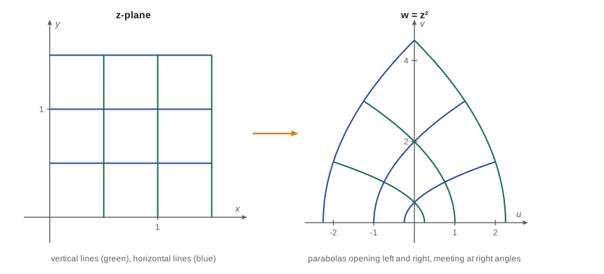
The map \(w = z^2\) is the first genuinely non-linear example. In polar form, \(re^{i\theta} \mapsto r^2 e^{2i\theta}\): moduli are squared and arguments doubled. So the ray at angle \(\theta\) goes to the ray at angle \(2\theta\), and a circle of radius \(r\) goes to a circle of radius \(r^2\), traced twice. The first quadrant \(0 < \theta < \frac{\pi}{2}\) is mapped onto the upper half-plane, and the upper half-plane onto the plane with the non-negative real axis removed. Because \(z\) and \(-z\) have the same square, the map is two-to-one away from the origin.

In Cartesian form, \(u = x^2 - y^2\) and \(v = 2xy\). The vertical line \(x = a\) becomes \(u = a^2 - y^2\), \(v = 2ay\); eliminating \(y = \frac{v}{2a}\) gives the parabola \(u = a^2 - \frac{v^2}{4a^2}\), opening to the left. The horizontal line \(y = b\) becomes the parabola \(u = \frac{v^2}{4b^2} - b^2\), opening to the right. The two families of parabolas cross at right angles, exactly as the grid lines they came from do. This is no accident: we will see in lesson 4 that analytic functions preserve angles wherever their derivative is non-zero. At the origin, where the derivative \(2z\) vanishes, angles are doubled instead: the right angle between the positive axes becomes the straight angle between the positive and negative real axes.

Inversion

The map \(w = \frac{1}{z}\), defined for \(z \ne 0\), sends \(re^{i\theta}\) to \(\frac{1}{r}e^{-i\theta}\). It is the composition of inversion in the unit circle, \(z \mapsto \frac{z}{|z|^2}\), which moves each point along its ray to the reciprocal distance, followed by conjugation. Points near 0 go to points far away and vice versa; the unit circle maps to itself, with the upper half going to the lower half.

The remarkable fact about inversion is that it maps circles and lines to circles and lines. To see it, note that every circle or line in the plane has an equation \(A(x^2 + y^2) + Bx + Cy + D = 0\) with real coefficients, a line when \(A = 0\). In terms of \(z\), this is \(A|z|^2 + \operatorname{Re}(\bar{\beta}z) + D = 0\) with \(\beta = B + iC\). Substituting \(z = \frac{1}{w}\) and multiplying by \(|w|^2\) gives \(A + \operatorname{Re}(\bar{\beta}\bar{w}) + D|w|^2 = 0\), an equation of the same form in \(w\) with the roles of \(A\) and \(D\) swapped. So circles through the origin (\(D = 0\)) map to lines, and lines not through the origin map to circles through the origin. For example, the line \(\operatorname{Re} z = 1\) maps to the circle \(|w - \frac{1}{2}| = \frac{1}{2}\).

The extended plane and the point at infinity

Inversion suggests adding a single point \(\infty\) to the plane, with \(\frac{1}{0} = \infty\) and \(\frac{1}{\infty} = 0\). The result, \(\hat{\mathbb{C}} = \mathbb{C} \cup \{\infty\}\), is the extended complex plane. Riemann pictured it as a sphere: place a sphere of radius 1 on the plane with its south pole at 0, and join each point \(z\) of the plane to the north pole by a straight line. The line meets the sphere at one other point, and this stereographic projection matches the plane with the sphere minus the north pole. Points far from the origin correspond to points near the north pole, so the north pole itself is \(\infty\). On the Riemann sphere, lines in the plane are simply circles that pass through \(\infty\), which explains why lines and circles behave alike under inversion. We say \(f(z) \to \infty\) as \(z \to z_0\) if \(|f(z)|\) grows without bound, and \(f(z) \to L\) as \(z \to \infty\) if \(f(\frac{1}{t}) \to L\) as \(t \to 0\).

The exponential map, a preview

Lesson 5 defines \(e^z = e^x(\cos y + i\sin y)\) for \(z = x + iy\). As a mapping it sends the horizontal line \(y = b\) to the ray from the origin at angle \(b\), and the vertical segment \(x = a\), \(-\pi < y \le \pi\), to the circle of radius \(e^a\). So it turns Cartesian coordinates in the \(z\)-plane into polar coordinates in the \(w\)-plane, mapping the horizontal strip \(-\pi < y \le \pi\) one-to-one onto the plane minus the origin. Because \(e^{z + 2\pi i} = e^z\), it is periodic with period \(2\pi i\), and infinitely many points share each image. Its inverse, the logarithm, must therefore be multi-valued, and taming that multi-valuedness is the subject of lesson 5.

Mappings of regions

Often we want a function that maps one region onto another. Typical tools are linear maps to move and scale, powers to open or close angles, inversion to turn circles into lines, and the exponential to turn strips into sectors. For example, to map the sector \(0 < \operatorname{Arg} z < \frac{\pi}{4}\) onto the upper half-plane, use \(w = z^4\), which multiplies angles by 4. To map the strip \(0 < \operatorname{Im} z < \pi\) onto the upper half-plane, use \(w = e^z\): the line \(y = 0\) goes to the positive real axis, the line \(y = \pi\) to the negative real axis, and every horizontal line in between to a ray in the upper half-plane. Lesson 12 develops this into a systematic method for solving problems in heat flow, electrostatics and fluid mechanics.

Experiments in Python

The code below maps grid lines through \(z^2\), checks that the line \(\operatorname{Re} z = 1\) goes under inversion to the circle of center \(\frac{1}{2}\) and radius \(\frac{1}{2}\), and tests a few points of the half-disk example.

import cmath, math

f = lambda z: z * z
# Vertical line x = 1: images should satisfy u = 1 - v^2/4.
for y in [-2, -1, 0, 0.5, 1.5]:
    w = f(complex(1, y))
    print(f"z = 1{y:+}i -> w = {w.real:+.2f}{w.imag:+.2f}i   1 - v^2/4 = {1 - w.imag**2/4:+.2f}")

# Inversion sends the line Re z = 1 to the circle |w - 1/2| = 1/2.
dev = max(abs(abs(1/complex(1, y) - 0.5) - 0.5) for y in [x/10 for x in range(-100, 101)])
print("largest deviation from the circle:", f"{dev:.1e}")

# Half-disk under z^2: moduli squared, arguments doubled.
for r, th in [(1, math.pi/6), (1.9, math.pi/2), (0.5, 0.95*math.pi)]:
    w = f(cmath.rect(r, th))
    print(f"r={r}, theta/pi={th/math.pi:.3f} -> |w|={abs(w):.3f}, arg/pi={(cmath.phase(w) % (2*math.pi))/math.pi:.3f}")

# The exponential sends the strip 0 < Im z < pi to the upper half-plane.
print([round(cmath.exp(complex(x, y)).imag, 3) > 0 for x in (-1, 0, 2) for y in (0.1, 1.5, 3.0)])

z = 1-2i -> w = -3.00-4.00i   1 - v^2/4 = -3.00
z = 1-1i -> w = +0.00-2.00i   1 - v^2/4 = +0.00
z = 1+0i -> w = +1.00+0.00i   1 - v^2/4 = +1.00
z = 1+0.5i -> w = +0.75+1.00i   1 - v^2/4 = +0.75
z = 1+1.5i -> w = -1.25+3.00i   1 - v^2/4 = -1.25
largest deviation from the circle: 1.1e-16
r=1, theta/pi=0.167 -> |w|=1.000, arg/pi=0.333
r=1.9, theta/pi=0.500 -> |w|=3.610, arg/pi=1.000
r=0.5, theta/pi=0.950 -> |w|=0.250, arg/pi=1.900
[True, True, True, True, True, True, True, True, True]

Common mistakes